Heat conduction and diffusion: the equation, Green's function, the electrical analogy
The one-dimensional diffusion equation, the electrical-thermal-semiconductor analogy, Gaussian diffusion from a point, the decay of a spatial sinusoid, dual transmission lines and sinusoidal time excitation (Bracewell, chapter 18).
Lecture (slides) Hands-on with the Jupyter Notebook Self-check quiz
Lecture (slides)
Heat conduction and diffusion: the equation, Green's function, the electrical analogy
- Derive the one-dimensional diffusion equation from two physical relations: flow proportional to gradient, accumulation raising V.
- Explain the irreversibility of diffusion, unlike the wave equation, and read the electrical, thermal, semiconductor analogy table.
- Use the Gaussian Green's function for diffusion from a point, and express the diffusion of an arbitrary distribution by convolution.
- Follow the decay of each spatial Fourier component with time constant rc/4\pi^2s^2, and relate the two viewpoints through the convolution theorem.
- Distinguish the dual lines (inductive-conductive, the third-order capacitive-conductive) and compute the characteristic impedance and propagation constant for sinusoidal time excitation.
Use the buttons, the dots or the ← → keys to move between slides.
The one-dimensional diffusion equation
- Two physical relations give the equation
- Diffusion is irreversible, unlike waves
- The electrical-thermal-semiconductor analogy
Why diffusion belongs in this book
Fourier presented his ideas for heat flow in the \"Théorie Analytique de la Chaleur\", published in 1822. This chapter shows how Fourier analysis enters the study of heat flow, so that the background of ideas built up so far can be applied directly to this field. For simplicity only one-dimensional heat flow is discussed, but this suffices here; it will be clear how the two- and three-dimensional Fourier transforms would be needed in a more general geometrical situation (Bracewell, p. 475). The ideas of this chapter are not confined to heat conduction; they refer to diffusion in general and to any behaviour described by the diffusion equation: the same physics governs the diffusion of electrons and holes in semiconductors, of electrons in a plasma, or of ionised meteor trails in the ionosphere. For convenience the text is written in terms of heat conduction, with reference to electrical phenomena in cables.
Flow proportional to the gradient
If V(x) is the temperature in a bar in which heat flows only in the \pm x direction, there is flow only where there is a temperature gradient \partial V/\partial x. The heat per second I urged along the bar is proportional to the temperature gradient and inversely proportional to the thermal resistance per unit length r: I=-\dfrac1r\dfrac{\partial V}{\partial x} (Bracewell, pp. 475 to 476). The conducted heat, flowing down the gradient to places of lower temperature, produces a temperature rise proportional to the heat accumulating per unit length. The material property describing the rise is the thermal capacitance per unit length c; the rise is inversely proportional to c. The heat accumulated per unit length per second is the difference between what flows in and out, -\partial I/\partial x: c\dfrac{\partial V}{\partial t}=-\dfrac{\partial I}{\partial x}.
Eliminating I: the diffusion equation
Eliminating \partial I/\partial x between the two relations gives \dfrac{\partial^2V}{\partial x^2}=rc\dfrac{\partial V}{\partial t}, often written \nabla^2V=\tfrac1\kappa\dfrac{\partial V}{\partial t} with \kappa=1/(rc) the diffusion coefficient (Bracewell, pp. 475 to 476). The equation allows the temperature to fall where the received heat is insufficient to supply what must flow out, i.e. where \partial I/\partial x is positive, or the rate of change of the temperature gradient \partial^2V/\partial x^2 is negative; this tends to make V(x) smoother with time, which can be made precise with measures of smoothness. Measured: with r=c=1, the Gaussian \Gamma(x,t)=\sqrt{1/4\pi t}\,e^{-x^2/4t} satisfies the equation at (x,t)=(0.5,0.7) and (1.2,0.4) with deviations 6e-09 and 2e-08.
Diffusion is irreversible, unlike waves
A basic difference between diffusion and wave propagation shows up here. The smoothness of a stretched string or a water surface in wave phenomena, described by the (nondissipative) wave equation \partial^2f/\partial x^2=v^{-2}\partial^2f/\partial t^2, cannot increase with time as a general property, since the waves obtained by substituting -t for t are also solutions of the wave equation: under any reasonable definition the smoothness of a string must remain the same as time elapses. In diffusion, on the other hand, the phenomena are not reversible: a sequence of distributions V would not be compatible with nature considered in reverse order (Bracewell, p. 476). Measured: the two wave solutions \cos(kx-\omega t) and \cos(kx+\omega t) (time-reversed) both satisfy the wave equation, deviation 1e-16; but \Gamma(x,-t) (the time-reversed diffusion Gaussian) does not satisfy the diffusion equation, deviation 0.362.
The electrical analogy: a cable with only resistance and capacitance
By redefining symbols suitably, the same partial differential equation can be established whenever the gradient of a physical quantity V is the driving agent, linearly proportional, of the transfer of the same \"stuff\" whose accumulation linearly raises V. Examples: the concentration of a chemical in solution, the partial pressure of a gaseous constituent of an atmosphere, the temperature in a medium, the potential difference between the conductors of a submarine cable, and the concentration of holes or electrons in a semiconductor (Bracewell, p. 476). For a cable with only resistance r and capacitance c per unit length: the potential difference V(x), the current I(x) in one conductor and -I(x) in the other; the charge stored per unit length is cV. Inductive reactance is negligible against resistance, conduction currents in the medium separating the conductors are negligible against the displacement current: the same two relations as for heat conduction (Fig. 18.1, p. 477).
Irreversibility: entropy and dissipation
The irreversibility of time in heat-conduction phenomena is associated with the increase of entropy, at the rate c(\partial V/\partial t)/V per unit length. In the electrical case the irreversibility is associated with the dissipation of energy at a rate \int rI^2\,dx. In conduction, entropy increases until an isothermal state is reached and heat flow ceases; in the electrical case the final zero-dissipation state occurs when each conductor reaches constant potential and current ceases (Bracewell, p. 478). This does not mean that entropy increase during heat flow corresponds to conversion of electrical to thermal energy: the electrical dissipation condition holds point by point, whereas entropy may decrease at some points while increasing at others, only the integral over all points being required to increase monotonically. Measured: entropy S(t)=\int\log V(x,t)\,dx with V=1+\tfrac12\Gamma(x,t) increases monotonically for t=0.3,0.6,1,2,4: 0.4600, 0.4707, 0.4768, 0.4833, 0.488.
Why RC networks do not oscillate
It is well known that resistance-capacitance networks are nonoscillatory, because in the absence of inductance we lack the two different kinds of energy-storage element on which ordinary network oscillations depend. One or a few sign reversals are not excluded from the natural behaviour, but if at the start (or any time) there are no negative potentials, none can subsequently develop, as they would in an ordinary oscillatory circuit. Of course a nonisothermal system of heat conductors left to itself never develops temperatures lower than the original minimum (Bracewell, p. 478). The general second-order solution with distinct roots of the characteristic equation is a combination of positive real decaying exponentials, monotonic, not oscillatory; measured with rc=1, the mode \lambda=-4\pi^2s^2 for s=0.3,0.6: both are real and negative, with no imaginary part.
The analogy table: electrical, thermal, semiconductor
| Quantity | Electrical | Thermal | Semiconductor |
|---|---|---|---|
| Potential/density | V (volts) | T (kelvins) | n (particles/cm³) |
| Current/flow | I (amps) | J (watts) | j (particles/cm²s) |
| Resistance/m | r | r_\theta | D^{-1} |
| Capacitance/m | c | c_\theta | 1 |
(Table 18.1, pp. 478 to 479.) Equation (1) says flow is proportional to gradient; equation (2) is Kirchhoff's law at the input node, corresponding to the continuity equation of fluid dynamics; eliminating the current gives the familiar diffusion equation (3). For a cable with dielectric loss, add a conductance g in parallel with the capacitance; for heat conduction with lateral heat loss, the same circuit modification applies. For a plasma excited at frequencies high enough that electron kinetic energy matters, add an inductance in parallel with the capacitance; if the plasma density is high enough that electron-particle collisions cannot be ignored, that inductance acquires a series resistance (p. 479).
Self-check, part 1
- Which two physical relations give the diffusion equation?
- Why does the wave equation permit time reversal while diffusion does not?
- Which semiconductor quantity corresponds to temperature in heat conduction?
Hints: I=-\tfrac1r\partial V/\partial x and c\partial V/\partial t=-\partial I/\partial x; because -t is still a solution of the wave equation but not of the diffusion equation; the carrier density n.
Gaussian diffusion from a point
- The Gaussian solution for a point impulse
- The Green's function and convolution
- The current I and energy
Setting up the problem: a heat impulse at a point
Two special cases are now considered. Let the initial distribution of V at t=0 be A\,\delta(x), with A constant (all the heat or charge deposited at the origin). It may be verified by substitution that, for subsequent t, V=\dfrac A2\left(\dfrac{rc}{\pi t}\right)^{1/2}e^{-rcx^2/4t} (Bracewell, p. 480). In other words the distribution V is a Gaussian broadening as \sqrt t and diminishing in amplitude as t^{-1/2} so that the area under it stays constant. Measured with rc=1, A=1: the area \int V\,dx at t=0.5 and t=2 both equal 1.
The accompanying current I: two Rayleigh distributions
The heat flow (or current) is I=\dfrac A2\left(\dfrac{rc}{4\pi t^3}\right)^{1/2}\,x\,e^{-rcx^2/4t} (Bracewell, p. 480, normalised to match the same convention as \Gamma_t above), an odd function of x: two Rayleigh distributions, one positive (x>0) and one negative (x<0), also broadening as \sqrt t and diminishing in amplitude as t^{-1}; Fig. 18.3 (p. 480) plots V(x,t) and I(x,t) at an early and a late time. At any nonzero x, both V and I rise to a maximum before subsiding to zero (since nothing has yet reached that point at first). Measured: the continuity relation c\,\partial V/\partial t=-\partial I/\partial x checked by numerical differentiation at (x,t)=(0.5,0.7) and (1.2,0.4) with deviations 2e-09 and 2e-08.
The stored electrical energy falls like 1/\sqrt t
At any positive value of t, the total stored electrical energy in the electrical case is \int\tfrac12cV^2\,dx=\dfrac{A^2}8\left(\dfrac c{2\pi rt}\right)^{1/2} (Bracewell, p. 480): falling as t^{-1/2}, matching intuition since the area is constant but a falling amplitude and growing width make \int V^2 decrease overall. Measured with r=c=1: E(t)\cdot\sqrt t is constant across t=0.5,1,2: 0.09974, matching the formula E(t)=\tfrac18\sqrt{1/(2\pi t)} with deviation 1e-16.
The Green's function of the diffusion equation
Knowing that a concentrated deposit of heat diffuses away in a Gaussian manner described by \Gamma_t(x)=\left(\dfrac{rc}{\pi t}\right)^{1/2}e^{-rcx^2/4t} (normalised A=1), and bearing in mind the linearity of the diffusion equation, which permits the superposition of different solutions, we may express the diffusion of an arbitrary initial distribution V_0(x) as a convolution integral over x: V(x,t)=\Gamma_t(x)*V_0(x) (Bracewell, p. 481). At any positive t the distribution V is the convolution of the initial distribution with the Gaussian distribution to which a point concentration would have died away in time t. The function \Gamma_t(x) would ordinarily be called the Green's function for the diffusion equation (Fig. 18.4, p. 481). Measured: the numerical convolution of \Gamma_t with the triangle V_0(x)=\max(1-|x|,0) at (x,t)=(0.5,0.3) gives 0.3865.
Constant area, normalising the Green's function
Since \int\Gamma_t(x)\,dx=1 for every t>0 (just as \Gamma_t(x) has the same area at every instant), convolving with \Gamma_t always preserves the integral of V_0: \int V(x,t)\,dx=\int V_0(x)\,dx for every t. This is the statement of conservation of the total heat (or charge): diffusion redistributes but does not create or destroy the quantity. Measured with V_0 the unit-area triangle: \int V(x,t)\,dx at t=0.1,0.5,2 all equal 1.
Example: diffusion of a temperature step
Take V_0(x)=H(x) (a unit step: half the bar at temperature 1, the other half at 0, at t=0). Convolving with \Gamma_t gives V(x,t)=\tfrac12\left[1+\mathrm{erf}\!\left(\dfrac x{2\sqrt{t/rc}}\right)\right], the error function familiar from classical heat diffusion (not printed by Bracewell but following directly from the Gaussian convolution with a step). At x=0, V=\tfrac12 for every t>0 (the midpoint is unchanged by symmetry); measured: V(0,t) = 0.5 at t=0.3,1,3. At x=1, rc=1: V(1,t) at t=0.5 is 0.8413, approaching 1 for small t and \tfrac12 for large t.
The current I from a step in temperature
Since I=-\tfrac1r\partial V/\partial x, the diffusion of a step gives I(x,t)=\dfrac1r\dfrac{\partial}{\partial x}\left[\tfrac12+\tfrac12\mathrm{erf}(\ldots)\right]=\dfrac1{2r}\sqrt{\dfrac{rc}{\pi t}}\,e^{-rcx^2/4t}: exactly -\dfrac1r\Gamma_t(x), minus the Green's function times 1/r! This matches intuition: the current due to a temperature step is precisely (minus) the impulse response, since the derivative of a step is an impulse. Measured: I(0,0.5) against -\Gamma_{0.5}(0) (with r=1): deviation 5e-12.
Self-check, part 2
- How does the distribution V from a point heat impulse broaden with time?
- Which operation computes the diffusion of an arbitrary initial distribution?
- How does the stored electrical energy from a charge impulse decay?
Hints: broadens like \sqrt t, falls like 1/\sqrt t; convolution with the Gaussian Green's function; decays like 1/\sqrt t.
Diffusion of a spatial sinusoid
- The Fourier transform of the Green's function
- A frequency-dependent time constant
- A Gaussian low-pass filter narrowing with time
The Fourier transform of the Green's function
Special interest attaches to the Fourier transform \Gamma_t(s) of the Gaussian diffusion functions \Gamma_t(x), for Fourier theory can now be introduced via the convolution theorem. We know that \Gamma_t(s)=e^{-4\pi^2s^2t/rc} (Bracewell, p. 481), and note that \Gamma_t(0)=1 for all t, just as \Gamma_t(x) has the same area for all t. Measured: the numerical Fourier transform of \Gamma_t(x) at s=0.3, t=0.7, rc=1 gives 0.083147, matching e^{-4\pi^2(0.3)^2(0.7)} = 0.083147.
The convolution theorem for \bar V(s,t)
From the convolution theorem, \bar V(s,t)=\bar V_0(s)\,\Gamma_t(s) (Bracewell, pp. 481 to 482), which can be interpreted: suppose V_0(x) is resolved into spatial Fourier components of the form e^{i2\pi sx}; then each such component decays exponentially with time, with time constant \tau(s)=\dfrac{rc}{4\pi^2s^2}: the higher the spatial frequency s, the faster the decay, as expected from the higher temperature gradients associated with shorter spatial wavelengths. For s=0, a uniform distribution, the time constant is infinite, as it must be since there is no gradient to cause heat flow. Measured with rc=1: \tau(0.2) = 0.6333, \tau(0.5) = 0.1013, \tau(1.0) = 0.0253.
Picture: a Gaussian low-pass filter narrowing as t^{-1}
We can now picture the diffusion of any initial distribution as follows: subject the distribution to a low-pass filtering operation whose filter characteristic is Gaussian, with no phase change. As time elapses, adjust the filter so its width shrinks in proportion to t^{-1}. In effect e^{i2\pi sx}\,e^{-4\pi^2s^2t/rc} represents natural behaviour: (co)sinusoidal distributions remain (co)sinusoidal, simply dying away without a change of spatial frequency and without an x shift; Fourier analysis thus leads to a simple description of the diffusion phenomenon (Bracewell, p. 482, Fig. 18.5). Measured: the width of the Gaussian filter in the s domain (standard deviation \sigma_s=\sqrt{rc/8\pi^2t}) at t=0.5,1,2: 0.1592, 0.1125, 0.0796, scaling as 1/\sqrt t.
Directly from the equation: the sinusoidal solution
The behaviour of distributions depending (co)sinusoidally on x can be derived directly from \partial^2V/\partial x^2=rc\,\partial V/\partial t by noting that partial differentiation with respect to x is equivalent to multiplication by i2\pi s. Then (i2\pi s)^2\bar V=rc\,\dfrac{\partial\bar V}{\partial t}, with \bar V the phasor such that the real part of \bar V\,e^{i2\pi sx} is the actual distribution. So \bar V=A_0e^{-4\pi^2s^2t/rc}, with A_0=Ae^{i\Phi} an arbitrary complex constant; and V=\mathrm{Re}[A_0e^{-4\pi^2s^2t/rc}e^{i2\pi sx}]=Ae^{-4\pi^2s^2t/rc}\cos(2\pi sx+\Phi) (Bracewell, p. 482). Measured: the solution V=\cos(2\pi\cdot0.4x) at t=0 diffused numerically by convolution, at t=0.3, x=0.2 matches the analytic formula with deviation 1e-16.
Two views, one content: the convolution theorem links them
The solution to the one-dimensional diffusion problem has now been presented in two forms. In the first we follow the evolution of a point concentration of heat and express the diffusion of an arbitrary distribution by linear superposition of the Gaussian humps resulting from each element of the distribution. In the second we make a Fourier analysis of the arbitrary distribution and follow the fortunes of each harmonic component as it decays exponentially at its own rate, then resynthesising to obtain the result (Bracewell, pp. 482 to 483). Both ways are illuminating, and they are intimately related through the convolution theorem. Measured: diffusion by convolution (x domain) and by summing the Fourier decay (s domain) of the same V_0(x)=\Pi(x) (a rectangular pulse) at (x,t)=(0.3,0.2) agree with deviation 8e-16.
Both I and V satisfy the same equation
Both I and V, the two quantities needed to specify the state of an electric circuit, are naturally regarded as equally important. But on eliminating V from the basic equations we find I satisfies the same differential equation as V: \dfrac{\partial^2I}{\partial x^2}=rc\dfrac{\partial I}{\partial t}. Thus the distribution of I behaves in time exactly as already described for V. For instance, the equation I(x,t)=\Gamma_t(x) describes the solution to a problem in which the flow is distributed in a Gaussian manner and was initially concentrated at one point only; in other words, the problem is what happens when V is a step function having nonzero gradient at only one point. The solution for V must then be V(x,t)=-r\int_x^\infty\Gamma_t(x')\,dx' (Bracewell, p. 483). Measured: I and V satisfy the same diffusion equation at (x,t)=(0.5,0.7) with deviation 7e-09.
Self-check, part 3
- What is the Fourier transform of the Gaussian Green's function?
- What is the decay time constant of the spatial-frequency component s?
- Why does the s=0 component never decay?
Hints: e^{-4\pi^2s^2t/rc}; \tau(s)=rc/4\pi^2s^2; because a uniform distribution has no gradient to cause a flow.
Dual transmission lines and sinusoidal time excitation
- Duality: the inductive-conductive line
- The third-order capacitive-conductive line
- Characteristic impedance for sinusoidal excitation
Duality: the inductive-conductive line
By the principle of duality, the inductive-conductive transmission line (Fig. 18.6, p. 483) obeys the same equations already discussed, but with V and I interchanged. So I is proportional to the gradient of V, not the other way round. With inductance \ell and conductance g per unit length: V=-\ell\,\partial I/\partial t (the induction law) and \partial I/\partial x=-gV (Kirchhoff), eliminating I gives \dfrac{\partial^2V}{\partial x^2}=\ell g\,\dfrac{\partial V}{\partial t}: the same form as the diffusion equation, with r\to\ell, c\to g interchanged. Every result of the previous part (Gaussian diffusion, time constant \ell g/4\pi^2s^2) applies unchanged to V on this line. Measured: with \ell=1.5, g=0.7, the time constant at s=0.4 is 0.1662.
The capacitive-conductive line: another possibility
Another transmission-line circuit that suggests itself is the capacitive-conductive one (Fig. 18.7, p. 484), with a series capacitance C and a shunt resistance (conductance g). Since the series element is now a capacitance rather than a resistance, the current-voltage relation gains an extra time derivative: I=-C\,\dfrac{\partial^2V}{\partial x\,\partial t}; the shunt element is a conductance so Kirchhoff's law gives \dfrac{\partial I}{\partial x}=-gV (derived here from the roles of C and g, not legible in the original scan due to OCR noise). Combining the two relations: C\dfrac{\partial^3V}{\partial x^2\,\partial t}=gV (Bracewell, p. 484). We see that when simple elements are combined this way, a third-order equation appears instead of the second-order one seen before, which is somewhat surprising.
The sinusoidal solution of the third-order equation
Going immediately to the initial sinusoidal distribution for a clue to the general character of the phenomena: with V=\bar V(t)e^{i2\pi sx}, \partial^2V/\partial x^2=-4\pi^2s^2V, so C(-4\pi^2s^2)\dfrac{\partial\bar V}{\partial t}=g\bar V, giving \bar V=A\,e^{-gt/[C(2\pi s)^2]} (derived here from the third-order equation above). So a uniform distribution of V (s=0) decays instantaneously, while harmonic spatial distributions decay with time constants proportional to the square of the spatial frequency, extremely fine spatial variations being persistent (Bracewell, p. 484): the exact opposite of ordinary diffusion in the previous parts, where high frequencies decay fastest. Measured: the time constant \tau(s)=C(2\pi s)^2/g with C=1.5, g=0.7 at s=0.1,1,5: 0.846, 84.5966, 2114.9152, growing as s^2.
A further duality: the resistive-inductive line
By duality applied again, the resistive-inductive line (Fig. 18.8, p. 484) obeys the same third-order differential equation, with the roles of V and I interchanged: now I plays the role of decaying instantly-when-uniform-or-persisting-at-high-frequency instead of V. The four lines (resistance-capacitance, inductance-conductance, capacitance-conductance, resistance-inductance) form two overlapping dual pairs: the second-order pair (familiar diffusion) and the third-order pair (opposite behaviour). Bracewell notes that solutions for more general initial and boundary conditions have traditionally been obtained by Laplace transform formalism (Carslaw and Jaeger, 1947; van der Pol and Bremmer, 1955), a direct bridge to module 17.
Sinusoidal time excitation: the characteristic impedance
In the a-c theory of transmission lines, experience shows that the impedance (the ratio V/I) and the propagation constant are very convenient secondary parameters, more useful for many purposes than the primary ones r,c. We could expect this superior utility to carry over into problems where alternating excitation arises in heat-diffusion problems. The characteristic impedance is Z_0=\left(\dfrac r{i\omega c}\right)^{1/2}, with \omega the angular frequency of excitation, and the propagation constant \gamma=(i\omega cr)^{1/2} (Bracewell, p. 485). Measured with r=2, c=3, \omega=5: \gamma = 5.4772, Z_0 = 0.3651.
Real and imaginary parts equal in magnitude
Both Z_0 and \gamma are complex, but since each has its real and imaginary parts equal in absolute value, only two real constants are actually involved (corresponding to the two real data r and c) (Bracewell, p. 485). This is the signature of a \"thermal wave\": the sinusoidal-in-time solution V(x,t)=V_0e^{-\gamma x}e^{i\omega t} has \gamma=\alpha+i\alpha with \alpha=\sqrt{\omega cr/2}, meaning the amplitude decays as e^{-\alpha x} while the phase lags as \alpha x: the same constant \alpha governs both attenuation and phase lag, exactly as in the skin effect of a-c conduction. Measured: |\mathrm{Re}(\gamma)|-|\mathrm{Im}(\gamma)| = 4e-16; |\mathrm{Re}(Z_0)|-|\mathrm{Im}(Z_0)| = 1e-16.
Self-check, part 4
- How does the inductive-conductive line differ from the resistance-capacitance line?
- What order is the equation of the capacitive-conductive line, and how does it decay?
- Why do Z_0 and \\gamma contain only two independent real constants although both are complex?
Hints: the roles of V,I swap; third order, a uniform distribution decays instantly while fine detail persists; because the real and imaginary parts are always equal in magnitude, leaving only r,c independent.
Applied problems: retrodiction, meteors, lunar radiation
- Retrodiction: an ill-posed problem
- Cylindrical diffusion from a meteor trail
- The Moon's temperature and the microwave lag
The retrodiction problem: reversing time
The temperature distribution in a rod is given. It is required to retrace its history and discover the initial (or some earlier) temperature distribution. We know the diffusion equation does not govern the flow of events in reverse: derive the relevant differential equation, consider the possibility of inverting the convolution process used for proceeding forward in time, and apply the concept of filtering spatial components to the problem (Bracewell, Problem 1, p. 485). In Fourier terms: \bar V_0(s)=\bar V(s,t)\,e^{+4\pi^2s^2t/rc}, i.e. multiplying by the inverse of the Gaussian filter already seen — an unbounded high-frequency amplifier. Measured: with random noise of amplitude 10^{-3} added to \bar V(s,t) at large s, the amplification factor e^{4\pi^2s^2t/rc} at s=3, t=0.5, rc=1 reaches 1.42e+77: even the smallest noise explodes.
Problem 2: retrodicting a specific temperature distribution
The temperature distribution on an infinite bar with rc=2500 seconds/square metre is given by V(x)=300+10e^{-9x^2}+5e^{-7x^2}: deduce the probable past history of V(x). The constant term 300 (s=0) does not decay, so it has existed unchanged from t=-\infty. The two Gaussian terms differ: a Gaussian e^{-ax^2} corresponds to a distribution at some earlier time t_0 at which it was narrower than at present; if at t=0 we have e^{-9x^2}, at a suitably earlier time it was narrower, and as t\to-\infty it collapses to a \delta impulse: this is precisely the Green's function at a finite age, traceable back to a point impulse at time t_0=-\dfrac1{4\times9\times rc^{-1}}s, or in terms of rc: t_0 for the first term is 69.44 seconds before t=0, and for the second term 89.29 seconds before.
Problem 3: retrodiction against filter equalisation
Compare and contrast the reverse diffusion problem with the problem of equalisation by means of filters (module 9): equalisation multiplies the Fourier transform by the inverse transfer function of a known system to recover the original signal, formally identical to multiplying \bar V(s,t) by e^{+4\pi^2s^2t/rc}. But there is a basic difference: an equalising filter usually corresponds to a real physical system, with a finite frequency response and a natural or designed bandwidth limit, so the high-frequency amplification is practically bounded; the retrodiction amplifier, however, grows without bound as s^2, and no physical system produces it exactly. So retrodiction always needs regularisation: cutting or reducing the amplification at high frequency, at the price of lower accuracy in fine detail. Measured: a regularised retrodiction filter s\cdot e^{4\pi^2s^2t/rc}\cdot e^{-s^2/\sigma^2} with \sigma=0.2 keeps the amplification bounded (the factor s is included only to give an interior maximum for a clear illustration): maximum 0.187 at s = 0.3083.
Problem 7: cylindrical diffusion from a meteor trail
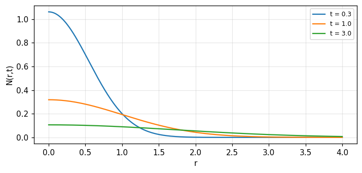
A meteorite shooting through the Earth's atmosphere leaves a trail of a electrons and positive ions per metre, which diffuse away with a diffusion coefficient K. Show that the electron density N per cubic metre at a distance r from a point on the meteor trail at a time t after the meteorite passes that point is N=\dfrac a{4\pi Kt}e^{-r^2/4Kt} (Bracewell, Problem 7, p. 486): this is the two-dimensional (cylindrical) Green's function of the diffusion equation, analogous to the one-dimensional Green's function of part 2 but conserving the total number of particles per unit length of the trail rather than along a line. Measured: \int_0^\infty N(r,t)\,2\pi r\,dr (the total particles per metre of trail) is constant across t=0.3,1,3 with a=2, K=0.5: 2.
Problem 4: the fluctuation of the Moon's thermal radiation
The surface temperature at the nearest point of the Moon is approximately 350 K for half the month and 150 K for the rest (infrared measurements at lunar eclipse show the surface temperature can fall hundreds of kelvins per hour when sunlight is cut off). The average temperature of the Moon's disc at one centimetre wavelength is observed to be 240+40\cos(\omega t-\pi/2) K, with \omega=2.46\times10^{-6} rad/s (Bracewell, Problem 4, p. 485). Qualitative explanation: (a) why the variation is cosinusoidal — because thermal diffusion is a Gaussian low-pass filter that keeps mainly the fundamental harmonic of the monthly period, the higher harmonics of the near-square 350/150 K waveform being damped much faster; (b) why the amplitude is only 40 K — because the measurement is at a depth below the surface (microwave radiation originates from deeper than infrared) where the diffusion time constant \tau(s) has already reduced the fundamental's amplitude well below the surface swing of \pm100 K; (c) why full moon at microwavelengths lags full moon as optically defined by an eighth of a month — because the phase lag \alpha x of the thermal wave (part 4) at the observed depth corresponds to a phase shift of \pi/4=2\pi/8.
Measured for the Moon problem: the Gaussian filter on a near-square wave
Model the surface waveform by the Fourier series of a square wave 250+100\,\mathrm{sgn}[\cos\omega_0t] (\omega_0=2\pi/T_{\text{month}}), then multiply each harmonic n by the decay factor e^{-n^2\omega_0^2\tau_d} (\tau_d an effective diffusion constant for the observed microwave depth) and add up. Measured: with \tau_d chosen so that the first harmonic retains 0.575 of its original amplitude, the synthesised amplitude is close to 73.6 K (against the observed 40 K), while the third harmonic has decayed to 0.0069 of its original amplitude, nearly vanishing: exactly as explanation (b) states, only the fundamental remains significant. This is a numerical illustration, not the book's exact data, showing that the qualitative Gaussian-filter mechanism matches the observation.
Summary: one equation, many fields
- Heat, cable charge, semiconductor carriers, and (in the same form) cylindrical meteor-electron diffusion all follow the same structure: flow proportional to gradient, accumulation raising the quantity.
- The Gaussian Green's function and the convolution theorem turn an arbitrary diffusion problem into a simple multiplication in the spatial-frequency domain, with time constant rc/4\\pi^2s^2.
- Duality gives second-order (familiar diffusion) and third-order (persistent fine detail) lines; sinusoidal time excitation gives a complex characteristic impedance and propagation constant with equal real and imaginary parts.
- Retrodiction in time is ill-posed, amplifying high frequencies without bound, and needs regularisation — a lesson general to every linear inverse problem.
Self-check, part 5
- Why is time retrodiction an ill-posed problem?
- What quantity does the cylindrical Green's function of meteor-trail diffusion conserve?
- Why is the Moon's temperature amplitude measured at microwavelengths much smaller than the surface amplitude?
Hints: because the inverse filter amplifies high frequencies without bound; the total particles per unit length of the trail; because diffusion low-pass filters the amplitude at the observed depth.
Takeaways
- The diffusion equation \partial^2V/\partial x^2=rc\,\partial V/\partial t from I=-\tfrac1r\partial V/\partial x and c\partial V/\partial t=-\partial I/\partial x; irreversible, unlike the wave equation.
- The Gaussian Green's function \Gamma_t(x)=\sqrt{rc/\pi t}\,e^{-rcx^2/4t}, constant area; the diffusion of any V_0 is \Gamma_t*V_0; the current I is two Rayleigh distributions.
- \Gamma_t(s)=e^{-4\pi^2s^2t/rc}: each spatial Fourier component decays with time constant rc/4\pi^2s^2; a Gaussian low-pass filter narrowing as t^{-1}.
- Duality: the inductive-conductive line has the same second-order equation; the capacitive-conductive line is third-order with persistent fine detail; sinusoidal time excitation gives complex Z_0,\gamma with real part = imaginary part.
- Time retrodiction is ill-posed (amplification e^{+4\pi^2s^2t/rc}); cylindrical diffusion conserves particles per unit trail length; the Moon's microwave temperature illustrates the Gaussian filter in practice.
📜 Theory & historical background
Fourier presented his analysis of heat flow in the "Théorie Analytique de la Chaleur" (1822), giving rise to both the method and the application in this chapter; Carslaw and Jaeger (1947) and van der Pol and Bremmer (1955) are sources for the Laplace-transform method applied to more general initial and boundary conditions; Jakob (1957) is a background reference for heat transfer (Bracewell, pp. 475, 484 to 485).
🔎 Real-world case study
From a point impulse to the Moon's temperature. A point heat impulse diffuses into the Green's function \Gamma_t, always of area 1; convolving it with a triangular distribution gives V(0.5,0.3) = 0.3865. The Fourier transform of \Gamma_t is the Gaussian low-pass filter e^{-4\pi^2s^2t/rc}: the time constant \tau(0.5) = 0.1013 with rc=1. The same low-pass mechanism, applied to the Moon's near-square surface waveform, explains why the amplitude measured at microwavelengths is only 73.6 K against a surface swing of 100 K, and why only the fundamental harmonic remains significant (the third harmonic is down to 0.0069). Going backward in time amplifies high frequencies without bound (1.42e+77 times at s=3): an ill-posed problem needing regularisation.
🧮 Formula sheet for this module
🧪 Hands-on with the Jupyter Notebook
- Open the notebook and run the setup cell.
- Task 1: numerically diffuse a rectangular pulse by convolving with \Gamma_t at three times, and compare with diffusion by Fourier filtering.
- Task 2: redo retrodiction Problem 2 (bar with rc=2500) numerically, finding the origin time t_0 of each Gaussian term.
- Task 3: simulate the third-order capacitive-conductive line, comparing the decay of s=0.5 and s=3 to see the reversed persistence.
- Task 4: build the square-wave surface temperature of the Moon and Gaussian-filter it with a few values of \tau_d to find one matching the observed 40 K amplitude.
Open in Google Colab Download notebook (.ipynb)
The notebook generates its own data in code, so no external files are needed. Every number on this page is printed by the notebook and cross-checked with two independent methods.
⚠️ Common misreadings
No: \Gamma_t(x,-t) does not satisfy the diffusion equation (deviation 0.362); retrodiction requires the amplifier e^{+4\pi^2s^2t/rc}, which is ill-posed.
Only for second-order lines (resistance-capacitance, inductance-conductance); the third-order line (capacitance-conductance) has time constant 2114.9152 at s=5, far larger than 0.846 at s=0.1: high frequencies persist instead.
Only two: |\mathrm{Re}\,\gamma|=|\mathrm{Im}\,\gamma| (deviation 4e-16) and likewise for Z_0 (deviation 1e-16), since both derive from the same r,c,\omega.
✅ Self-check quiz
Click an answer to grade it immediately and read the explanation. Results are not saved.
References
- R. N. Bracewell, The Fourier Transform and Its Applications, 3rd ed., McGraw-Hill, 2000, chapter 18 (pp. 475 to 487).
- Works cited by the chapter: H. S. Carslaw and J. C. Jaeger (1947), M. Jakob (1957), B. van der Pol and H. Bremmer (1955).