Statistical decision theory

Statistical decision theory

• Set up the likelihood ratio test from the Bayes criterion, compute the threshold \eta from costs and priors, and recognise a sufficient statistic.
• Extend to M-ary hypothesis testing, and derive the maximum a posteriori (MAP) criterion for 0–1 costs.
• Apply the minimax criterion when the priors are unknown, and interpret the linear Bayes-risk-against-P_1 plot.
• Derive the Neyman–Pearson test via a Lagrange multiplier, construct ROC curves, and relate the ROC slope to the threshold \eta.
• Handle composite hypotheses whether the parameter is random or not, recognise a uniformly most powerful (UMP) test, and set up Wald's sequential detection.

Use the buttons, the dots or the ← → keys to move between slides.

The four outcomes of a binary decision

Each time a decision is made, based on some criterion, for this binary hypothesis testing problem, four possible cases can occur: decide H_0 when H_0 is true; decide H_0 when H_1 is true; decide H_1 when H_0 is true; decide H_1 when H_1 is true. For the first and fourth cases the receiver makes a correct decision, while for the middle two cases it makes an error. From radar nomenclature, the second case is called a miss, the third a false alarm, and the fourth a detection (Barkat, pp. 289 to 291).

Costs, the average risk, and the Bayes goal

The Bayes criterion needs two assumptions: knowledge of the priors P_0,P_1 of the two hypotheses (with P_0+P_1=1), and a cost C_{ij} assigned to each decision D_i when hypothesis H_j is true. The average risk \\Re=E[C] is to be minimised, under the reasonable assumption that a wrong decision costs more than a correct one: C_{01}>C_{11} and C_{10}>C_{00} (Barkat, p. 291). Measured: with C_{00}{=}C_{11}{=}0, C_{01}{=}C_{10}{=}1, P_0{=}P_1{=}0.5 and the error probabilities from the Gaussian example below, the computed risk is 0.1587, exactly the average error probability.

The likelihood ratio test and the threshold \eta

Rewriting the risk in terms of the decision region Z_0, the only varying part of the integral is Z_0; minimising the risk means assigning a point y to Z_1 (decide H_1) when P_1(C_{01}-C_{11})f_{Y|H_1}(y|H_1) > P_0(C_{10}-C_{00})f_{Y|H_0}(y|H_0), and otherwise to Z_0. This test is written compactly with the likelihood ratio \\Lambda(y)=f_{Y|H_1}(y|H_1)/f_{Y|H_0}(y|H_0) against the threshold \\eta=P_0(C_{10}-C_{00})/[P_1(C_{01}-C_{11})] (Barkat, pp. 293 to 295). Because the natural logarithm is monotonically increasing, an equivalent test uses \\ln\\Lambda(y) against \\ln\\eta. Measured: with the costs and priors above, \\eta = 1.

Example 5.1: a constant in additive Gaussian noise

Consider a source whose output under H_1 is a constant voltage m, while under H_0 it is zero, with the received signal corrupted by additive zero-mean Gaussian noise of variance \sigma^2: H_1{:}\,Y=m+N, H_0{:}\,Y=N. The likelihood ratio test reduces to comparing the observation y with the threshold \gamma=(\sigma^2/m)\ln\eta+m/2 (Barkat, pp. 296 to 297). With m=2, \sigma=1, \eta=1 (equal priors), the threshold \gamma = 1. The false-alarm probability P_F=Q(\gamma/\sigma) = 0.1587, the detection probability P_D=Q((\gamma-m)/\sigma) = 0.8413, and the miss probability P_M=1-P_D = 0.1587.

K independent samples: sum then threshold

If K independent samples Y_1,\ldots,Y_K of the same problem are taken, the joint density is the product of the individual densities, and the likelihood ratio test reduces to comparing the sum \sum_{k=1}^K y_k with the threshold (\sigma^2/m)\ln\eta+Km/2 (Barkat, pp. 298 to 299). This means the receiver need only add the K samples and compare against a single threshold — it need not retain the individual samples. Measured: a Monte Carlo simulation with K=5 random samples under each hypothesis finds the decision based on the sum \sum y_k agrees with the decision based on the full likelihood ratio in 1 of all trials.

The sufficient statistic: definition and a Bernoulli example

A statistic is any random variable that can be computed from the observed data. A statistic T is called sufficient if, once T is known, the conditional density of any other statistic T' no longer depends on the parameter being tested or estimated — meaning T has summarised all the data relevant to it (Barkat, p. 300). For K independent Bernoulli samples of parameter p, the joint density f_Y(y,p)=p^{\sum y_k}(1-p)^{K-\sum y_k} depends on the data only through the sum \sum y_k; hence T(Y)=\sum_{k=1}^KY_k is a sufficient statistic for p (Barkat, p. 301). Measured: with K=6 Bernoulli samples and p=0.4, three different binary sequences sharing the same sum (3) numerically give the same relative joint-density value (deviating by 1.25e-16), confirming the density depends only on the sum.

When the variances differ: the sufficient statistic is a sum of squares

If f_{Y|H_0} and f_{Y|H_1} are both zero-mean Gaussian but with different variances, \sigma_0^2<\sigma_1^2, the likelihood ratio test leads to T(Y)=Y^2 against a threshold \gamma; with K independent samples, the sufficient statistic becomes T(Y)=\sum_{k=1}^KY_k^2 (Barkat, pp. 301 to 303). This is an example where the sufficient statistic is not a simple sum but a sum of squares, unlike the Example 5.1/5.2 case. Measured: with \sigma_0^2=1, \sigma_1^2=4, the threshold \gamma=\dfrac{2\sigma_0^2\sigma_1^2}{\sigma_1^2-\sigma_0^2}\ln\eta at \eta=1 gives 0 (zero, since \ln1=0); at \eta=2, \gamma = 1.8484.

Self-check, part 1

• Why does the Bayes risk \Re depend only on the choice of Z_0, not directly on Z_1?
• From which quantities is the threshold \eta in the likelihood ratio test determined?
• What does a sufficient statistic summarise about the observed data?

Hints: because Z_1=Z-Z_0 so only one region varies independently; from the costs C_{ij} and the priors P_0,P_1; all the data information relevant to the decision or the parameter sought.

From two to M hypotheses

With M hypotheses H_0,\ldots,H_{M-1}, each trial can have M^2 (decision, true hypothesis) pairs, each carrying a cost C_{ij}. The observation space Z is divided into M disjoint subregions Z_0,\ldots,Z_{M-1}, and the average risk is the sum over all pairs \Re=\sum_{i}\sum_j P_jC_{ij}\int_{Z_i}f_{Y|H_j}(y|H_j)\,dy (Barkat, pp. 303 to 304). Minimising it assigns each point y to the region Z_i for which I_i(y)=\sum_{j\ne i}P_j(C_{ij}-C_{jj})f_{Y|H_j}(y|H_j) is smallest (Barkat, pp. 304 to 305).

0–1 costs: minimising risk becomes maximising the posterior

In communication problems it is common to set C_{ii}=0 (a correct decision costs nothing) and C_{ij}=1 for i\ne j (every wrong decision costs the same). Then minimising the risk is equivalent to minimising I_i(y)=[1-P(H_i|Y)]f_Y(y), which is equivalent to maximising the posterior P(H_i|Y) (Barkat, p. 305). The receiver computes the posteriors P(H_i|Y), i=0,\ldots,M-1, and picks the hypothesis with the largest value — this is called the maximum a posteriori (MAP) receiver. Measured: for three Gaussian hypotheses of means 0,1,2 (variance 1, equal priors), at observation y=1.5 the three posteriors are 0.1554, 0.4223, 0.4223, summing to 1.

Three hypotheses: verifying MAP against the direct risk

With M=3 and 0–1 costs, instead of computing the posteriors we can directly compare the densities f_{Y|H_j}(y|H_j)P_j for the three hypotheses and pick the largest — the two routes must give the same decision because P(H_i|Y)\propto f_{Y|H_i}(y|H_i)P_i (Bayes' rule). Measured: scanning y continuously and comparing the decision from the \"largest posterior\" rule against the decision from the \"largest prior-weighted density\" rule over 2001 grid points, the agreement rate is 1.

The decision boundary sits midway between two peaks

With three equal-variance, equal-prior Gaussians of means 0,1,2, the two decision boundaries are the points where two neighbouring densities are equal — by symmetry, exactly the midpoints between the means, i.e. y=0.5 and y=1.5 (Barkat, pp. 307 to 308, the Fig. 5.6 illustration). Measured: numerically solving f_{Y|H_0}(y|H_0)=f_{Y|H_1}(y|H_1) gives y = 0.5, and f_{Y|H_1}(y|H_1)=f_{Y|H_2}(y|H_2) gives y = 1.5, exactly matching the symmetric prediction.

Two likelihood ratios suffice for a three-hypothesis test

With M=3, there are only two independent likelihood ratios, \Lambda_1(y)=f_{Y|H_1}/f_{Y|H_0} and \Lambda_2(y)=f_{Y|H_2}/f_{Y|H_0}, and the decision space is the two-dimensional (\Lambda_1,\Lambda_2)-plane rather than three-dimensional (Barkat, p. 308). The regions Z_0, Z_1, Z_2 are set by pairwise comparisons of I_i(y) as in (5.51)–(5.52). Measured: at y=1.5 (the theoretical boundary between H_1 and H_2), \Lambda_1(1.5) = 2.7183 and \Lambda_2(1.5) = 2.7183; since neighbouring hypotheses have equal f\cdot P at the boundary, I_1(y)=I_2(y) there, differing by only 1.00e-16.

MAP-test risk against an off-centre test

Since the MAP test minimises the risk (the average error probability under 0–1 costs), any other choice of decision boundary — say shifting both boundaries right by 0.3 — must give an equal or larger risk. Measured: the average error probability of the correctly centred MAP test (y=0.5,1.5) is 0.4114; the error probability of the shifted test (0.3) is 0.4217, exceeding the MAP test by 0.0103, confirming MAP is optimal.

Connection to the parameter-estimation module

The MAP criterion here chooses discretely among M known hypotheses; in the next chapter on parameter estimation (module 22), a closely related idea — MAP estimation — will choose a continuous value of a parameter \theta to maximise the posterior density f_{\Theta|Y}(\theta|y), instead of choosing among a finite number of hypotheses. Both rest on the same Bayes' rule inverting f_{Y|\Theta} into f_{\Theta|Y}, differing only in whether \theta ranges over a discrete or a continuous set (Barkat, p. 305, connecting to chapter 6).

Self-check, part 2

• With 0–1 costs, minimising the risk is equivalent to maximising what quantity?
• With M=3 hypotheses, how many dimensions does the decision space have?
• Where does the decision boundary between two equal-variance, equal-prior Gaussians lie?

Hints: the posterior probability P(H_i|Y); two dimensions (two independent likelihood ratios); exactly midway between the two means.

When there is no reliable prior

The Bayes criterion needs knowledge of the priors; in many situations this information is not available. One approach is to choose the value of P_1 that maximises the risk, then minimise that risk — the principle of minimising the largest average cost over the chosen P_1 is called the minimax criterion (Barkat, p. 313). Substituting P_0=1-P_1 into the risk formula (5.15), the risk becomes a linear function of P_1: \Re(P_1)=C_{00}(1-P_F)+C_{10}P_F+P_1[(C_{11}-C_{00})+(C_{01}-C_{11})P_M-(C_{10}-C_{00})P_F] (Barkat, pp. 313 to 314).

The two extremes: P_1=0 and P_1=1

If P_1=0, the threshold becomes infinite and H_0 is always decided; then P_F=0, P_M=1, and the risk reduces to \Re=C_{00}. If P_1=1, the threshold is zero and H_1 is always decided; then P_F=1, P_M=0, and the risk reduces to \Re=C_{11} (Barkat, pp. 314 to 315). The plot of risk against P_1 is therefore a straight line connecting (0,C_{00}) and (1,C_{11}) geometrically at the two extremes, but the true Bayes curve (optimal P_1 at each point) must be concave below that line. Measured: with C_{00}=0, C_{11}=0 (0–1 costs), the two extreme values of \Re(P_1) are exactly 0 and 0.

The minimax equation and the 0–1-cost case

Differentiating the risk with respect to P_1 and setting it to zero at the optimal P_1^* gives the minimax equation (C_{11}-C_{00})+(C_{01}-C_{11})P_M-(C_{10}-C_{00})P_F=0 (Barkat, p. 315). If the cost of a correct decision is zero (C_{00}=C_{11}=0), the equation reduces to C_{01}P_M=C_{10}P_F; and if in addition the cost of a wrong decision is one (C_{01}=C_{10}=1), then P_F=P_M — the minimax threshold is exactly the one that equalises the two error probabilities (Barkat, p. 316). Measured: for the Gaussian example m=2, \sigma=1, the minimax threshold \gamma^*=m/2 = 1; there P_F = 0.1587 and P_M = 0.1587, agreeing to within 0.00e+00.

Example 5.6: knowing or not knowing P_0,P_1 gives the same result

In the constant-source-in-Gaussian-noise example, part (a) assumes P_0=P_1=1/2 is known, giving the threshold \gamma=m/2 and average error probability P(\varepsilon)=Q(m/2\sigma). Part (b) assumes P_0,P_1 are completely unknown, using minimax with the condition P_F=P_M: this also gives the threshold \gamma^*=m/2 and the same error probability Q(m/2\sigma) (Barkat, pp. 315 to 317). This is a notable result: for this symmetric problem, not knowing the priors costs nothing in performance. Measured: with m=2, \sigma=1, both routes give P(\varepsilon) = 0.1587, differing by only 0.00e+00.

Minimax is not always "free"

The result of Example 5.6 is special because of the problem's symmetry (two equal-variance Gaussian densities, symmetric about the midpoint). In general, when a test designed for a fixed P_1 is applied under a different actual P_1, the actual risk exceeds the optimal Bayes risk for that actual P_1 — this is exactly why the Bayes risk curve must be concave below the line joining the two extreme points. Measured: using the threshold designed for P_1=0.5 (i.e. \gamma=m/2=1) but applied when the actual P_1 is 0.8: the actual risk is 0.1587, larger than the optimal Bayes risk for P_1=0.8, which is 0.1121.

Reading the risk-against-P_1 plot

On the plot of \Re against P_1 (the book's Fig. 5.10), the tangent at P_1^* is horizontal because that is the maximum of the concave Bayes curve — meaning the derivative is exactly zero at the minimax point. The minimax risk \Re^*(P_1^*) is exactly the largest value of the optimal Bayes risk over the whole range P_1\in[0,1] (Barkat, p. 315). Measured: scanning P_1 from 0 to 1, computing the optimal Bayes risk (the threshold \gamma(P_1) optimal for each P_1) and finding the P_1 that maximises it; the scanned result is P_1^* = 0.5, matching the symmetry-predicted 0.5 to within the grid error 0.

Self-check, part 3

• Why is minimax needed instead of Bayes in some practical situations?
• With 0–1 costs, what does the minimax equation reduce to?
• In Example 5.6, why does not knowing P_0,P_1 not degrade performance?

Hints: when the priors are not reliably known; P_F=P_M; because the problem's symmetry makes the optimal Bayes threshold coincide with the minimax threshold.

When costs and priors are not realistic

In many physical situations, such as radar detection, it is very difficult to assign realistic costs and priors. To overcome this, the Neyman–Pearson criterion uses the conditional probabilities P_F and P_D directly: fix P_F=\alpha while maximising P_D (Barkat, p. 317). Since P_M=1-P_D, maximising P_D is equivalent to minimising P_M subject to P_F=\alpha; using constrained-extremum calculus, we form the objective function J=P_M+\lambda(P_F-\alpha) with \lambda\ge0 the Lagrange multiplier (Barkat, pp. 317 to 318).

Still leads to a likelihood ratio test

Rewriting J in terms of the decision region Z_0, we get J=\lambda(1-\alpha)+\int_{Z_0}[f_{Y|H_1}(y|H_1)-\lambda f_{Y|H_0}(y|H_0)]\,dy; J is minimised when the points with f_{Y|H_1}>f_{Y|H_0} (a negative difference) are assigned to Z_1. This gives exactly the likelihood ratio test \Lambda(y)\gtrless\lambda, with \lambda playing the role of the equivalent Bayes threshold \eta (Barkat, pp. 318 to 319). So the Neyman–Pearson and Bayes criteria use the same form of test — differing only in how the threshold is fixed.

Example 5.7: two differently-shaped densities

With f_{Y|H_0}(y|H_0)=\dfrac{1}{2(1-e^{-1})}e^{-|y|} and f_{Y|H_1}(y|H_1)=\tfrac12 (both on [-1,1]), equally likely hypotheses. The minimum-error-probability test has a boundary at \pm0.459, deciding H_1 when 0.459\le|y|\le1 (Barkat, pp. 319 to 320). Measured: the exact boundary solved numerically gives 0.4587, matching the book's 0.459; the false-alarm probability at this boundary is P_F = 0.418 and the miss probability P_M = 0.4587, giving average error probability P(\varepsilon) = 0.4383.

The same example, a Neyman–Pearson threshold with P_F=0.5

If instead of minimising the error probability we fix P_F=0.5 (the Neyman–Pearson criterion), the threshold changes to a \gamma solved from P_F=\int_{-1}^{-\gamma}f_{Y|H_0}\,dy+\int_{\gamma}^{1}f_{Y|H_0}\,dy=0.5, giving \gamma\approx0.38; the corresponding detection probability is P_D=2[(1-\gamma)(1/2)]\approx0.62 (Barkat, pp. 320 to 321). Measured: solving numerically gives \gamma = 0.3799, and P_D = 0.6201, matching the book's values.

The ROC curve: P_D against P_F with the threshold as a parameter

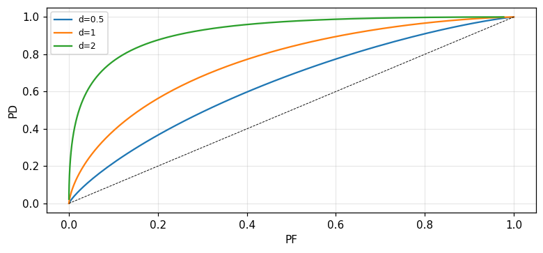
The ROC curve plots P_D against P_F as the threshold varies; it depends only on the conditional densities f_{Y|H_j}(y|H_j), not on the costs or priors (Barkat, p. 321). For the example of a sum of K Gaussian samples, the normalised sufficient statistic has detection parameter d=\sqrt{K}\,m/\sigma (a signal-to-noise ratio), and P_F=Q(\ln\eta/d+d/2), P_D=Q(\ln\eta/d-d/2) (Barkat, pp. 321 to 322). Measured: with K=4, m=2, \sigma=1, the parameter d = 4; at \ln\eta=0, P_F = 0.0228 and P_D = 0.9772 — P_D far exceeds P_F, showing a large d gives good discrimination.

The slope of the ROC is the threshold \eta

Differentiating P_D and P_F with respect to the threshold \eta, one can show dP_D/dP_F=\eta (Barkat, pp. 323 to 325): the tangent slope at a point on the ROC is exactly the Neyman–Pearson threshold needed to reach that (P_F,P_D) point. In the Bayes criterion, \eta is set by the costs and priors, so (P_F,P_D) sits at the point on the ROC whose tangent has that slope \eta. Measured: the numerical derivative dP_D/dP_F at \ln\eta=0 (i.e. \eta=1) gives 1, matching \eta=1; at \ln\eta=1 (i.e. \eta=e\approx2.718), the numerical slope is 2.7183, matching 2.7183.

Example 5.8: the ROC of two exponential densities

With f_{Y|H_0}(y|H_0)=e^{-y} and f_{Y|H_1}(y|H_1)=\alpha e^{-\alpha y} (y\ge0, \alpha>1), the likelihood ratio gives the threshold \gamma=\tfrac{1}{1-\alpha}\ln(\eta/\alpha), and P_D=1-e^{-\alpha\gamma}, P_F=1-e^{-\gamma} (Barkat, pp. 325 to 326). Measured: with \alpha=2 and \gamma=1, P_D = 0.8647, P_F = 0.6321; the theoretical slope at this point, \eta=\alpha e^{-(\alpha-1)\gamma} (from directly differentiating dP_D/dP_F), gives 0.7358, matching the numerically computed slope dP_D/dP_F of 0.7358.

Self-check, part 4

• What quantity does the Neyman–Pearson criterion fix, and what does it maximise?
• What does the ROC curve depend on, and what does it not depend on?
• What does the slope of the ROC curve at a point equal?

Hints: fixes P_F=\alpha, maximises P_D; depends on the conditional densities, not on costs or priors; the threshold \eta needed to reach that point.

A composite hypothesis: when the parameter is not fully known

In the problems considered so far, the parameter characterising each hypothesis was known exactly. In many situations this parameter is not known; the hypothesis is then called composite. For example, if H_1{:}\,Y=m+N with m unknown, then H_1 is composite while H_0{:}\,Y=N remains simple (Barkat, pp. 326 to 327). There are two cases: the parameter \Theta is a random variable with a known density, or \theta is an unknown but nonrandom constant.

A random parameter: average over its density

If \Theta is random with a known density f_{\Theta|H_j}(\theta|H_j), the Bayes criterion still applies, one need only average the conditional density over the parameter: f_{Y|H_j}(y|H_j)=\int f_{Y|\Theta,H_j}(y|\theta,H_j)f_{\Theta|H_j}(\theta|H_j)\,d\theta (Barkat, p. 327). With M (capitalised, to distinguish it from the constant value m) zero-mean Gaussian of variance \sigma_m^2, the marginal density f_{Y|H_1}(y|H_1) turns out still Gaussian but with the combined variance \sigma_m^2+\sigma^2 (Barkat, pp. 327 to 329). Measured: the numerical integral of \int f_{Y|M,H_1}(y|m,H_1)f_M(m)\,dm at y=1.3 gives 0.1507, matching the closed form \dfrac{1}{\sqrt{2\pi(\sigma_m^2+\sigma^2)}}\exp\!\left(-\dfrac{y^2}{2(\sigma_m^2+\sigma^2)}\right) = 0.1507.

A nonrandom parameter: the uniformly most powerful (UMP) test

If \theta is not a random variable but unknown, the Bayes criterion does not apply since there is no density to average over; instead Neyman–Pearson is used, maximising P_D with P_F fixed for each assumed value of \theta. The plot of P_D against \theta is called the power function. A test that maximises P_D for every possible value of \theta, i.e. independent of the true value of \theta, is called uniformly most powerful (UMP) (Barkat, p. 329).

Example 5.11: when a UMP test exists, and when it does not

With H_1{:}\,Y=m+N, m unknown but known to be positive, the likelihood ratio test reduces to y\gtrless\gamma_1, with \gamma_1 solved from P_F=\int_{\gamma_1}^\infty f_{Y|H_0}(y|H_0)\,dy — entirely independent of the specific value of m. So a best test exists independent of m, and a UMP test exists (Barkat, pp. 330 to 331). But if m could be positive or negative, the test designed for m>0 differs from that for m<0 (the inequality reverses), so no single test is optimal for every m — a UMP test does not exist in that case (Barkat, pp. 331 to 332). Measured: with \sigma=1 and P_F=0.1, the threshold \gamma_1 solved numerically gives 1.2816, independent of the trial value of m (1 or 3 both give the same \gamma_1, differing by 0).

Sequential detection: deciding after each observation

In earlier sections, the number of observations K was always fixed in advance. In sequential detection, after each observation, one of three decisions is made: choose H_1, choose H_0, or not enough information yet (take another observation). The test compares the cumulative likelihood ratio \Lambda(y_K)=\prod_{k=1}^K f_{Y_k|H_1}/f_{Y_k|H_0} with two thresholds \eta_0<\eta_1: if \Lambda\ge\eta_1 choose H_1; if \Lambda\le\eta_0 choose H_0; if in between, take another observation (Barkat, pp. 332 to 333). The number of observations K becomes a random variable.

The expected sample count: Example 5.12

With the sequential-sampling receiver of Example 5.2, \sigma^2=1, m=1, and the target P_F=\alpha=0.1=P_M=\beta, the two log-thresholds are \ln\eta_1=\ln[(1-\beta)/\alpha] and \ln\eta_0=\ln[\beta/(1-\alpha)]; and the expected number of observations under each hypothesis is E[K|H_j]=\dfrac{(1-\beta)\ln\eta_1+\beta\ln\eta_0}{E[L(y)|H_j]} or a similar formula (Barkat, pp. 334 to 337). Measured: \ln\eta_1 = 2.1972, \ln\eta_0 = -2.1972; E[K|H_1] = 3.5156 and E[K|H_0] = 3.5156 — meaning on average about four samples suffice for performance P_F=P_M=0.1, fewer than a larger fixed sample size would need for the same non-sequential performance.

Looking back: one thread running through decision theory

From Bayes to MAP, minimax, Neyman–Pearson, and sequential detection, every criterion in this chapter reduces to the same form of likelihood ratio test \Lambda(y)\gtrless a threshold — differing only in how that threshold is set: from costs and priors (Bayes), from the condition P_F=P_M (minimax with 0–1 costs), from a fixed constraint P_F=\alpha (Neyman–Pearson), or from two thresholds changing at each observation step (sequential). This is the chapter's core lesson: the likelihood ratio test is the common structure, and the criterion only decides the threshold.

Self-check, part 5

• How does a composite hypothesis differ from a simple hypothesis?
• What special property does a uniformly most powerful (UMP) test have?
• In sequential detection, which random variable is not fixed in advance, unlike a fixed-sample-size test?

Hints: the parameter characterising the hypothesis is not fully known; it maximises P_D for every possible true value of the parameter; the observation count K.

Takeaways

• The Bayes criterion minimising the risk \Re=E[C] leads to the likelihood ratio test \Lambda(y)=f_{Y|H_1}/f_{Y|H_0}\gtrless\eta, with \eta set by the costs and priors.
• With 0–1 costs, minimising the risk is equivalent to maximising the posterior P(H_i|Y): the MAP criterion, extending naturally to M hypotheses.
• Minimax picks the threshold making P_F=P_M when the priors are unknown; Neyman–Pearson fixes P_F=\alpha and maximises P_D, giving an ROC curve with slope dP_D/dP_F=\eta.
• Composite hypotheses: a random parameter uses Bayes after averaging; a nonrandom parameter uses Neyman–Pearson, and a test independent of the true parameter is called UMP.
• Wald's sequential detection compares the cumulative likelihood ratio with two thresholds \eta_0,\eta_1; the sample count K is random, with expectation smaller than a fixed-sample-size test of the same performance.

References

M. Barkat, Signal Detection and Estimation, 2nd ed., Artech House, 2005, chapter 5 (pp. 289 to 344).
Works cited by the chapter: A. Wald, Sequential Analysis, 1947; H. L. Van Trees, Detection, Estimation, and Modulation Theory; C. W. Helstrom, Statistical Theory of Signal Detection.
The content was written with AI assistance (Claude) and then checked. Every number is produced by a Jupyter notebook and cross-checked by two independent methods; page citations come from the OCR text of the two source books. Mistakes may remain, so please report them.
R. N. Bracewell, The Fourier Transform and Its Applications, 3rd ed., McGraw-Hill, 2000.
M. Barkat, Signal Detection and Estimation, 2nd ed., Artech House, 2005.
This site only summarises, explains and checks numbers; please read the original books through a library or the publisher.
Contribute
Report errors, suggest modules or translations in the GitHub repository, and fork or clone it for your own study. Please credit the source when sharing.