Electromagnetic Compatibility (EMC) in Aircraft
Tooley ch.14 (p.218-237) · Lecture "EMC and Aircraft" (46 slides) · Floyd ch.13 section 13-1, ch.6 section 6-11, ch.15 section 15-3
📚 Chapter mapping: 9 lectures ↔ textbook chapters
Tooley: Ch.14 EMC (p.218-237): 14.1 harmonics and pulse spectrum, 14.2 EMC and avionic equipment, 14.3 spectrum analysis (noise floor, Table 14.1 bands), 14.4 effects, sources and reduction of EMI, 14.5 wiring, 14.6 grounding and bonding; 9 MCQs (A.14, p.381)
Floyd: Floyd has NO EMC chapter. Only partial matches: Ch.13 section 13-1 (cross talk, UTP/STP twisted pairs against EMI, p.741), Ch.6 section 6-11 (VCC-to-ground decoupling, p.364), Ch.15 section 15-3 (noise margin, p.859; Problem 3 p.887). Most of the module relies on Tooley and the lecture.
The 46-slide lecture (each slide read) has 3 dB exercise sets (slides 17, 19, 21); all were re-solved and the 10 kW versus 100 kW error on slide 21 was caught. The module has 3 interactive demos (dB and dBm, square-wave Fourier, a real capacitor) and records the mismatches found in the material.
Opening case: Wi-Fi and the Boeing 757 cockpit displays
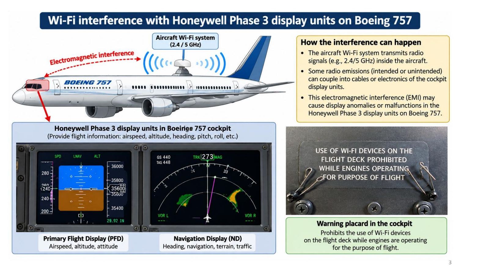
The aircraft Wi-Fi system transmits at 2.4 or 5 GHz. Some of the emissions (intended or not) can couple into the wiring or electronics of the Honeywell Phase 3 displays (PFD, ND) in the Boeing 757 cockpit and cause display anomalies. Hence the cockpit placard banning Wi-Fi devices while the engines run for the purpose of flight.
Definition of EMC
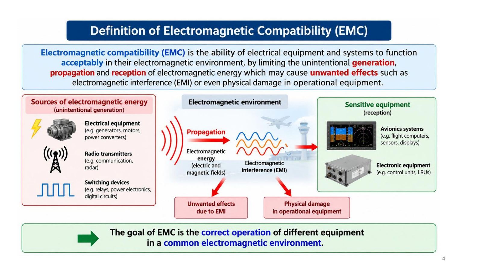
Electromagnetic compatibility (EMC) is the ability of electrical equipment and systems to function acceptably in their electromagnetic environment by limiting the unintentional generation, propagation and reception of electromagnetic energy that may cause unwanted effects such as electromagnetic interference (EMI) or even physical damage. The goal: different equipment working correctly in a common electromagnetic environment.
The electromagnetic environment of an aircraft
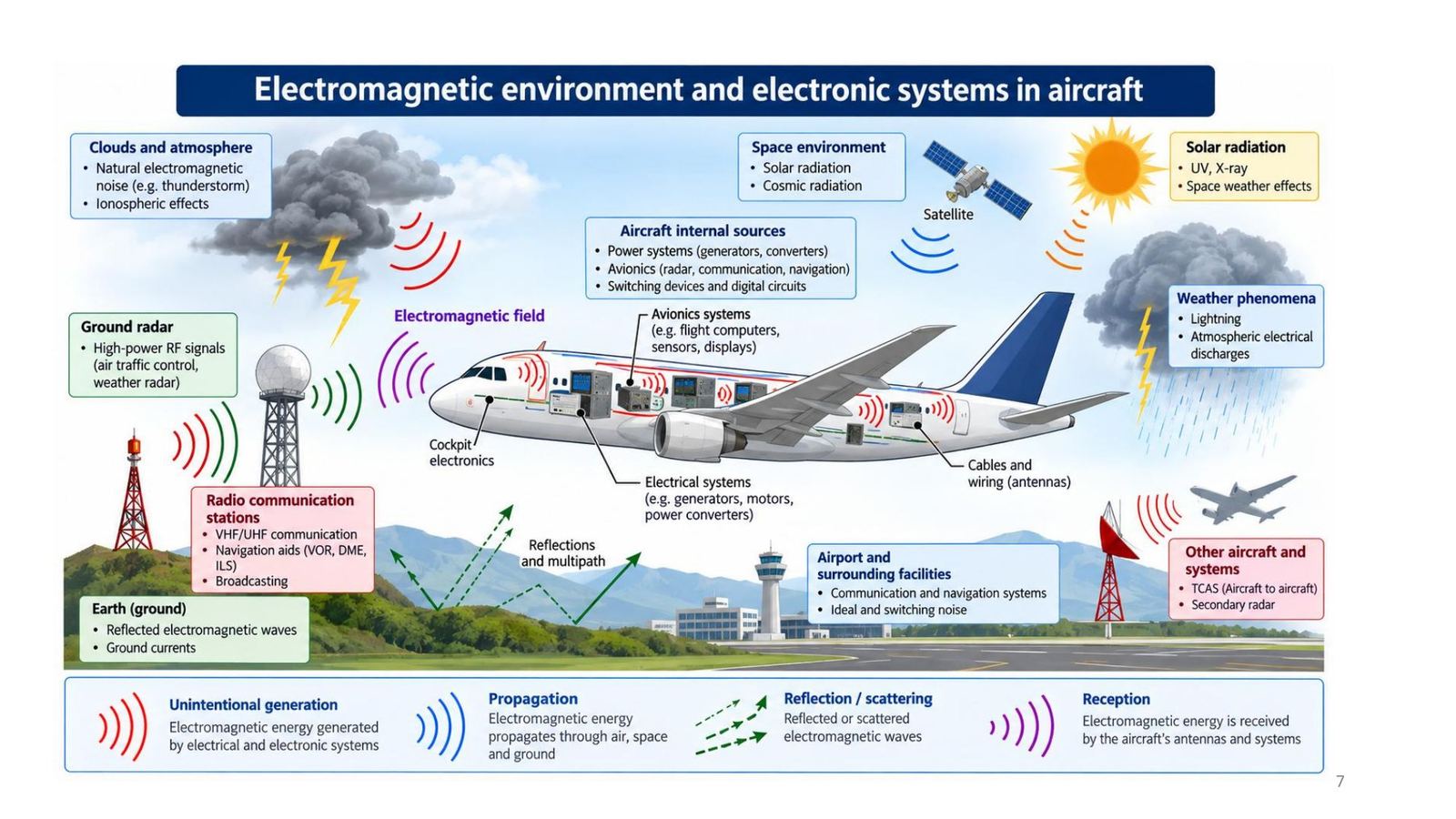
External sources: lightning and weather, ground radar, VHF/UHF and navigation radio stations (VOR, DME, ILS), other aircraft (TCAS), solar and cosmic radiation. Internal sources: generators, motors, converters, avionics and switching devices. Four steps of the energy: unintentional generation, propagation, reflection/scattering, reception (through the aircraft's antennas and wiring).
Strength of electromagnetic sources
| Source | Field strength (slide) |
|---|---|
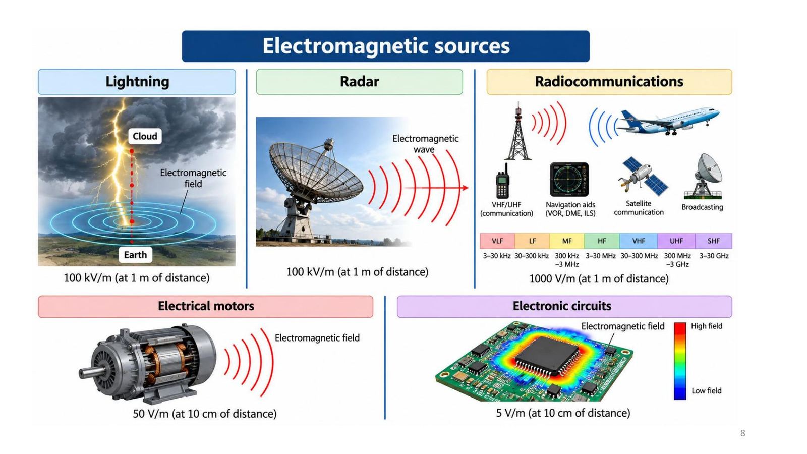
| Lightning | 100 kV/m at 1 m |
| Radar | 100 kV/m at 1 m |
| Radio communication | 1000 V/m at 1 m |
| Electric motor | 50 V/m at 10 cm |
| Electronic circuit | 5 V/m at 10 cm |
Bands: VLF 3 to 30 kHz, LF 30 to 300 kHz, MF 300 kHz to 3 MHz, HF 3 to 30 MHz, VHF 30 to 300 MHz, UHF 300 MHz to 3 GHz, SHF 3 to 30 GHz.
Signal types in EMC
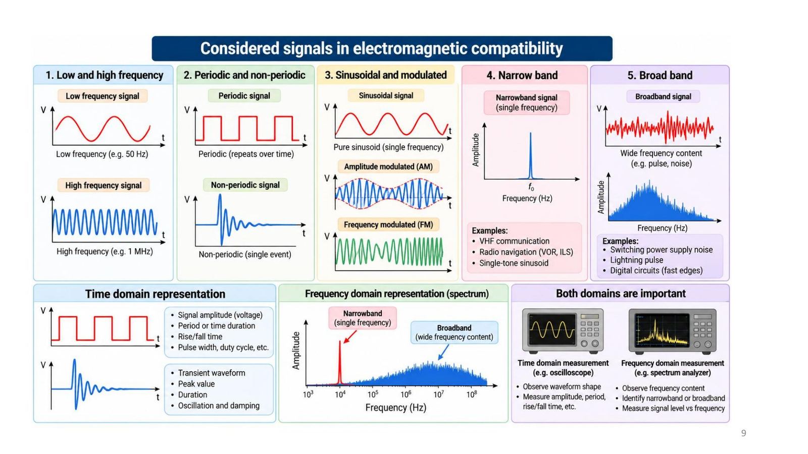
All waveforms must be considered: low and high frequency, periodic and non-periodic, sinusoidal and modulated (AM, FM), narrowband (one frequency: VHF, VOR/ILS) and broadband (pulses, noise: switching supplies, fast-edge digital circuits, lightning pulses).
Time domain (oscilloscope): amplitude, period, rise and fall time. Frequency domain (spectrum analyser): frequency content, narrowband or broadband, level versus frequency.
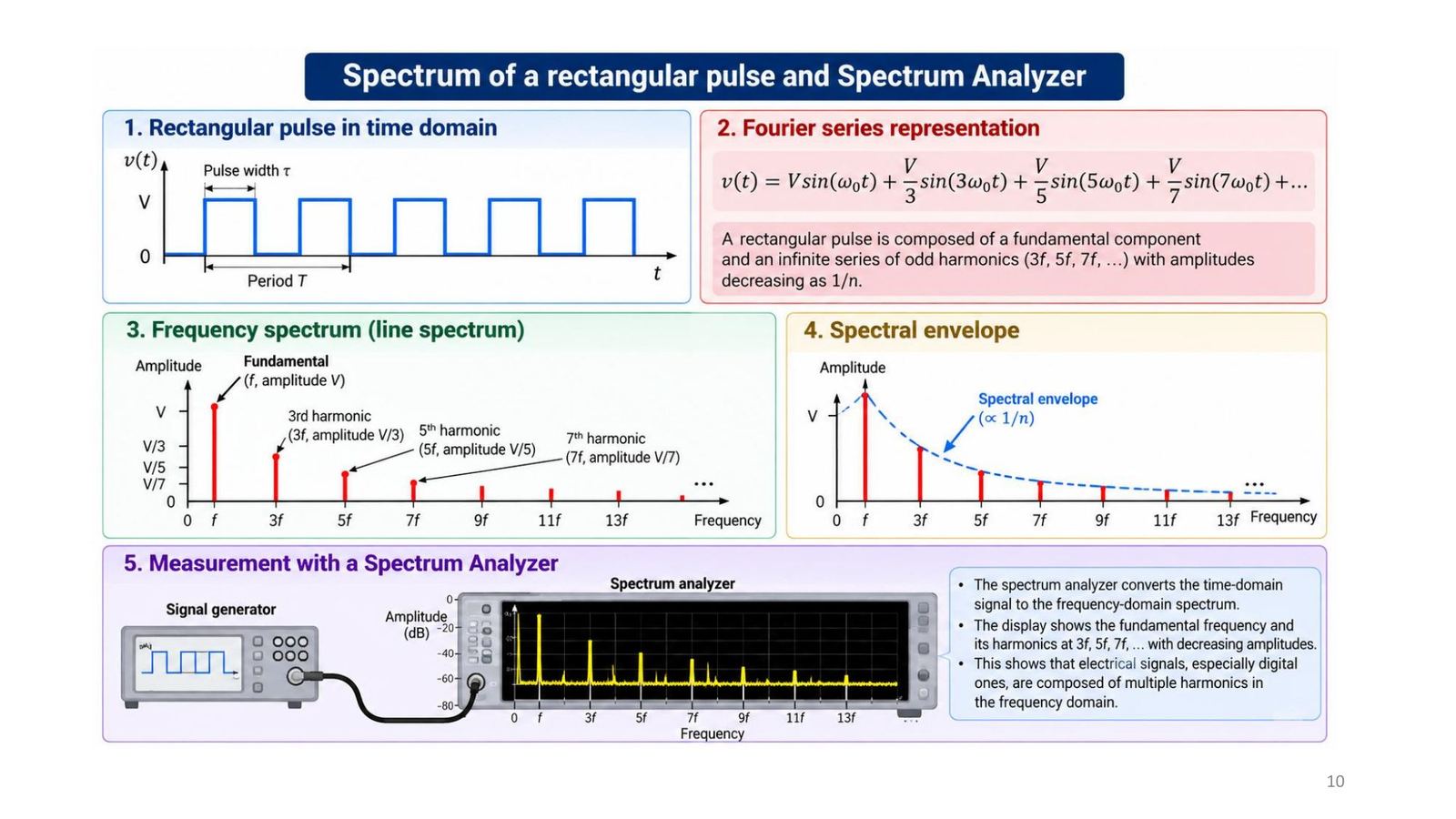
Spectrum of a rectangular pulse: a sum of odd harmonics
Every complex wave comprises a fundamental plus many harmonics, each with its own amplitude and phase (Fourier analysis). Square wave: v = V[sin ωt + (1/3) sin 3ωt + (1/5) sin 5ωt + (1/7) sin 7ωt + …], only odd harmonics (f, 3f, 5f, 7f, …) with amplitude V/n; the spectral envelope is proportional to 1/n. Try Demo 2 at the bottom of the page.
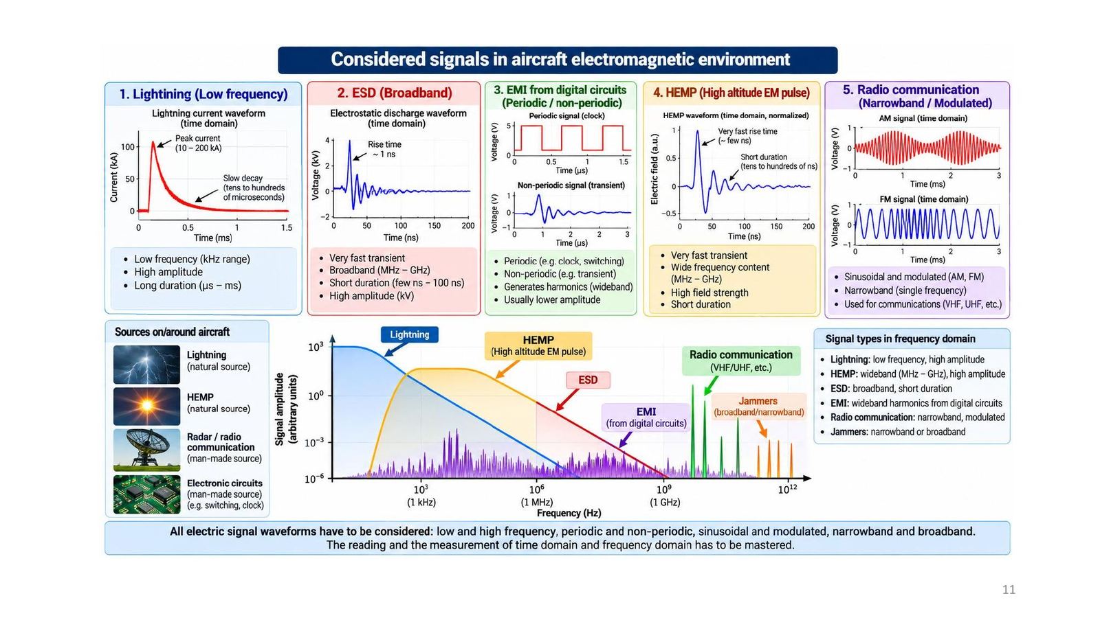
Signals in the aircraft electromagnetic environment
| Source | Characteristics |
|---|---|
| Lightning | Low frequency (kHz), very high amplitude (peak 10 to 200 kA), µs to ms long |
| ESD | Broadband (MHz to GHz), rise time about 1 ns, kV, short (few ns to 100 ns) |
| Digital-circuit EMI | Periodic and non-periodic, generates wideband harmonics, lower amplitude |
| HEMP | Very fast, wide frequency content (MHz to GHz), high field strength, short |
| Radio | Narrowband, modulated (VHF, UHF) |
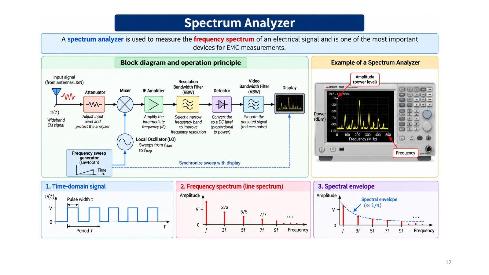
The spectrum analyser
A spectrum analyser measures the frequency spectrum of an electrical signal and is one of the most important devices for EMC measurements. Block diagram (lecture): attenuator → mixer → intermediate-frequency (IF) amplifier → resolution bandwidth filter RBW → detector → video bandwidth filter VBW → display; the local oscillator LO sweeps from f_start to f_stop in sync with the display.
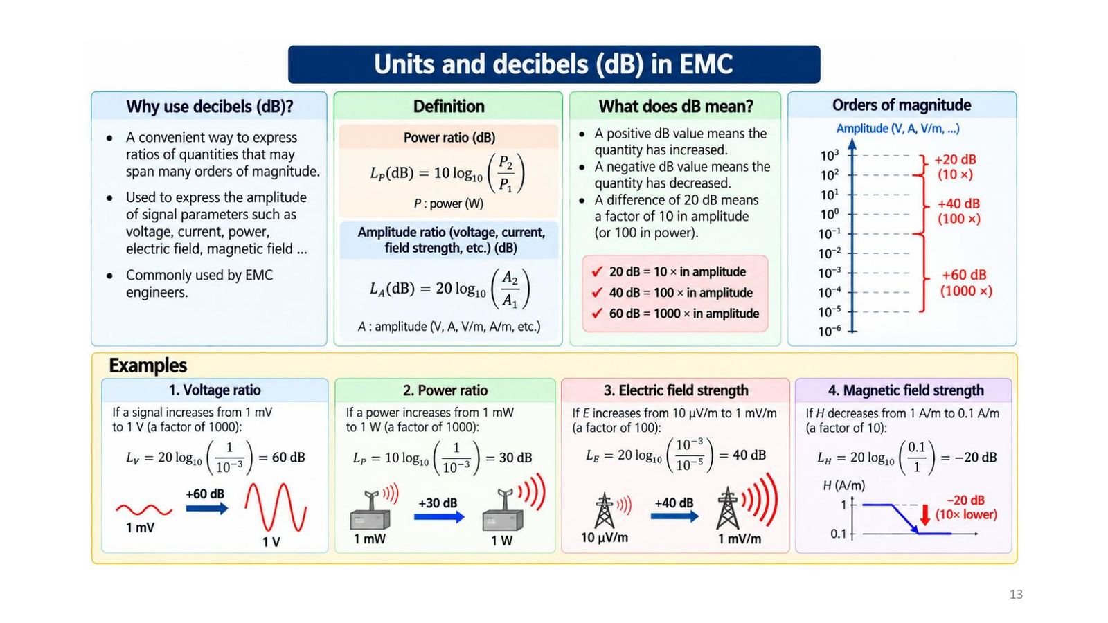
Why use dB
The dB is a compact way to express ratios of quantities spanning many orders of magnitude, used for the amplitude of voltage, current, power, electric and magnetic field. Rules: a positive dB value means an increase, a negative one a decrease; 20 dB = 10 × amplitude, 40 dB = 100 ×, 60 dB = 1000 × (or 100, 10,000, 1,000,000 × in power).
Examples: 1 mV to 1 V = +60 dB; 1 mW to 1 W = +30 dB; 10 µV/m to 1 mV/m = +40 dB; H from 1 to 0.1 A/m = −20 dB.
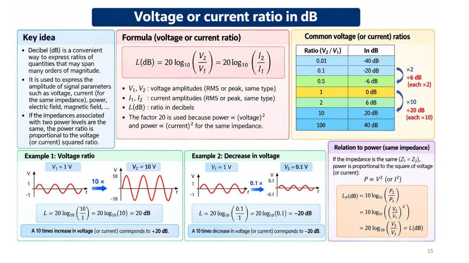
Power ratio and voltage ratio
| Power ratio | dB | Voltage ratio | dB |
|---|---|---|---|
| 0.01 | −20 | 0.01 | −40 |
| 0.1 | −10 | 0.1 | −20 |
| 0.5 | −3 | 0.5 | −6 |
| 1 | 0 | 1 | 0 |
| 2 | 3 | 2 | 6 |
| 10 | 10 | 10 | 20 |
| 100 | 20 | 100 | 40 |
L_P = 10 log(P₂/P₁); L = 20 log(V₂/V₁) = 20 log(I₂/I₁) because P ∝ V² (same impedance).
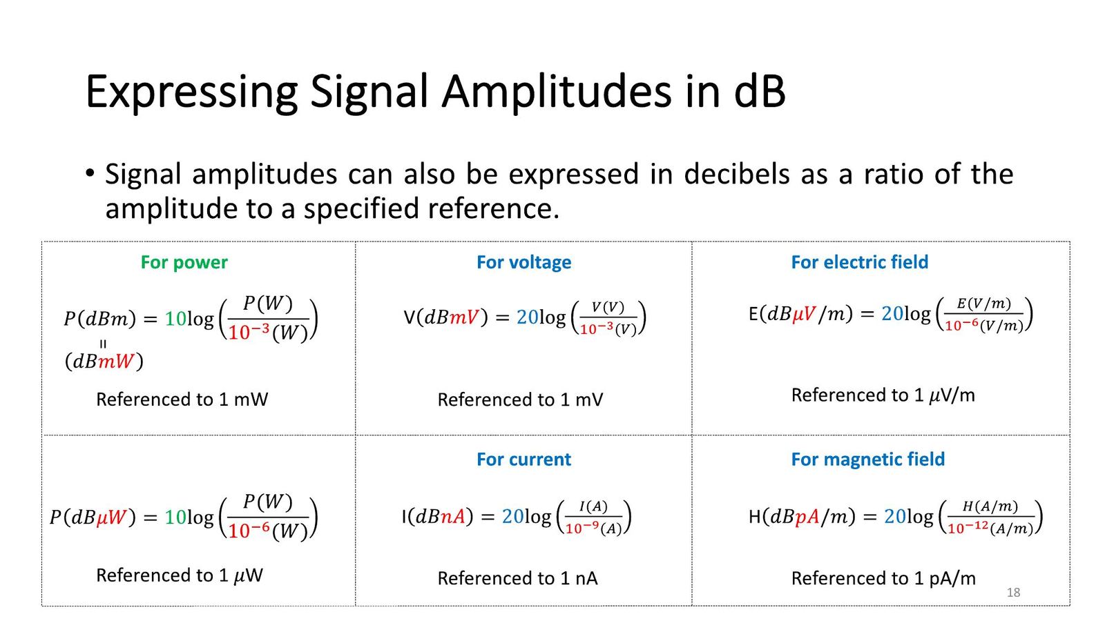
Absolute amplitudes: dBm, dBµV, dBµV/m
| Quantity | Formula | Reference |
|---|---|---|
| Power | P(dBm) = 10 log(P/10⁻³ W) | 1 mW |
| Power | P(dBµW) = 10 log(P/10⁻⁶ W) | 1 µW |
| Voltage | V(dBmV) = 20 log(V/10⁻³ V) | 1 mV |
| Electric field | E(dBµV/m) = 20 log(E/10⁻⁶ V/m) | 1 µV/m |
| Current | I(dBnA) = 20 log(I/10⁻⁹ A) | 1 nA |
| Magnetic field | H(dBpA/m) = 20 log(H/10⁻¹² A/m) | 1 pA/m |
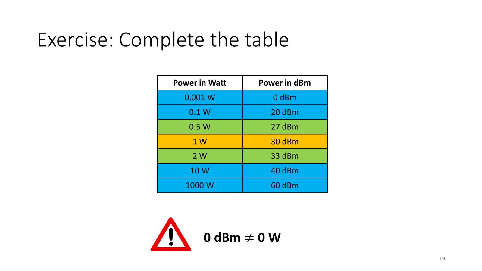
Exercises on slides 17 and 19: dB ratios and the dBm table
| Ratio (slide 17) | Formula | dB |
|---|---|---|
| 200 : 100 µV/m | 20 log 2 | 6.02 |
| 300 : 100 mV | 20 log 3 | 9.54 (≈ 10) |
| 400 : 100 mA | 20 log 4 | 12.04 |
| 500 : 100 µA/m | 20 log 5 | 13.98 (≈ 14) |
| 2 : 1 µW | 10 log 2 | 3.01 |
| 3 : 1 mW | 10 log 3 | 4.77 (≈ 5) |
| 5 : 1 mW | 10 log 5 | 6.99 (≈ 7) |
Slide 19 table: 0.001 W = 0 dBm; 0.1 W = 20; 0.5 W = 27; 1 W = 30; 2 W = 33; 10 W = 40; 1000 W = 60 dBm.
Adding and subtracting dB: gain and loss chains
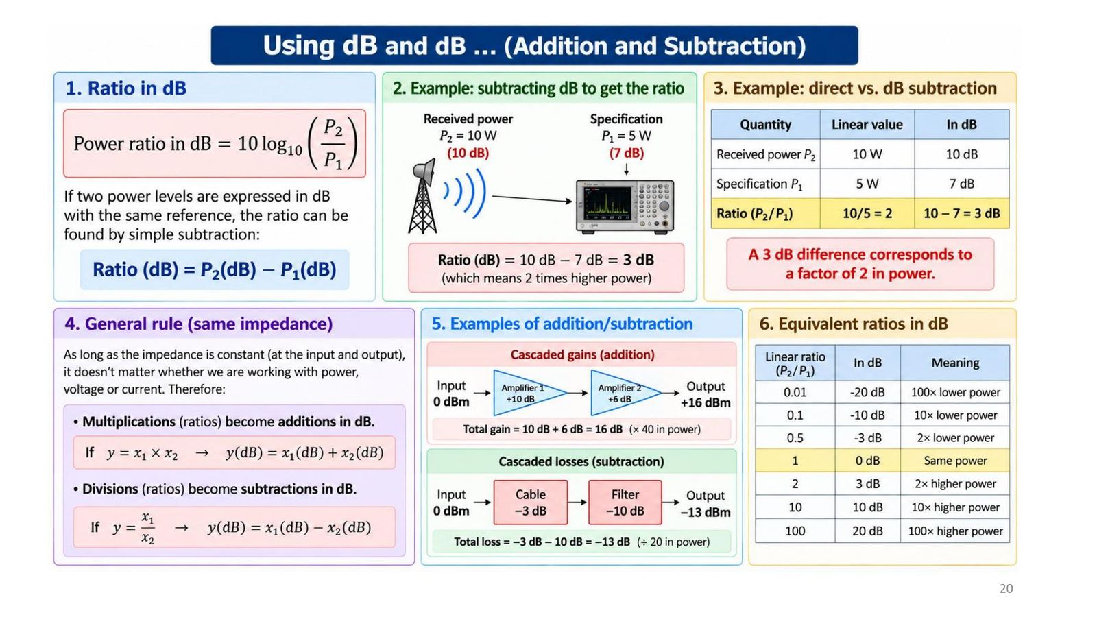
With the same impedance, multiplying ratios becomes adding dB and dividing becomes subtracting dB. Two levels with the same reference can be subtracted: Ratio(dB) = P₂(dB) − P₁(dB); e.g. receiving 10 W (10 dB) against a 5 W specification (7 dB) gives 3 dB, i.e. double. Chains: 0 dBm through +10 dB and +6 dB amplifiers gives +16 dBm; 0 dBm through a −3 dB cable and a −10 dB filter gives −13 dBm.
Exercises on slide 21: four step-by-step solutions
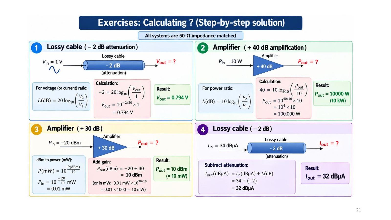
| # | Task | Result |
|---|---|---|
| 1 | Cable −2 dB, V_in = 1 V | V_out = 10^(−2/20) = 0.794 V |
| 2 | Amplifier +40 dB, P_in = 10 W | P_out = 10 × 10⁴ = 100,000 W (100 kW) |
| 3 | +30 dB, P_in = −20 dBm | P_out = 10 dBm (= 10 mW) |
| 4 | Cable −2 dB, I_in = 34 dBµA | I_out = 32 dBµA |
What EMC standards contain
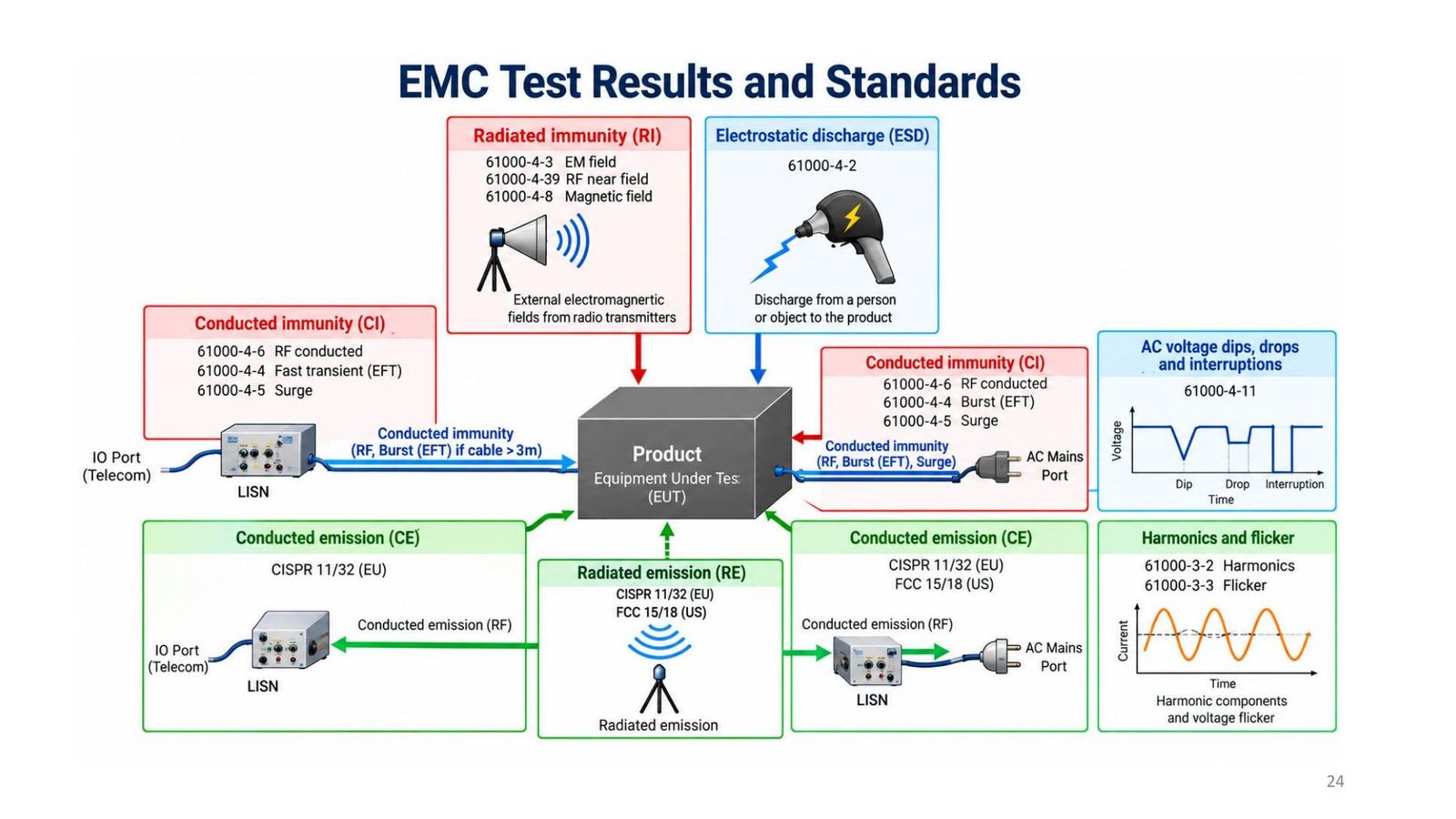
An EMC standard = terms and definitions + rules and requirements + test methods + limits and minimum test levels. Two groups: emissions (limit the unwanted electromagnetic energy the product emits, conducted and radiated) and immunity (the product works correctly under external disturbance: ESD, radiated RF field, fast transient EFT/burst, surge, conducted RF).
| Emission | Immunity |
|---|---|
| CISPR 32: multimedia equipment | IEC 61000-4-2: ESD |
| CISPR 11: industrial, scientific, medical (ISM) equipment | IEC 61000-4-3: radiated RF field; -4-4: EFT/burst; -4-5: surge |
Example limit: CISPR 11 (Group 1, Class A)
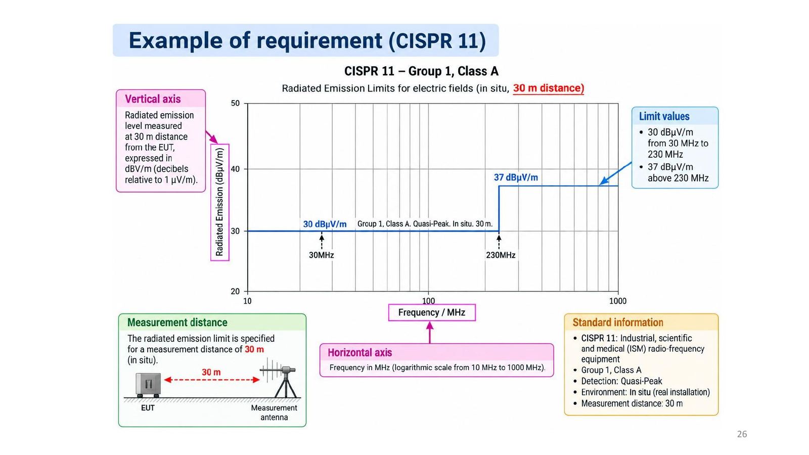
Radiated emission limit for the electric field, measured in situ at 30 m with a quasi-peak detector: 30 dBµV/m from 30 MHz to 230 MHz and 37 dBµV/m above 230 MHz. The vertical axis is dBµV/m (relative to 1 µV/m), the horizontal axis is frequency on a logarithmic scale from 10 to 1000 MHz.
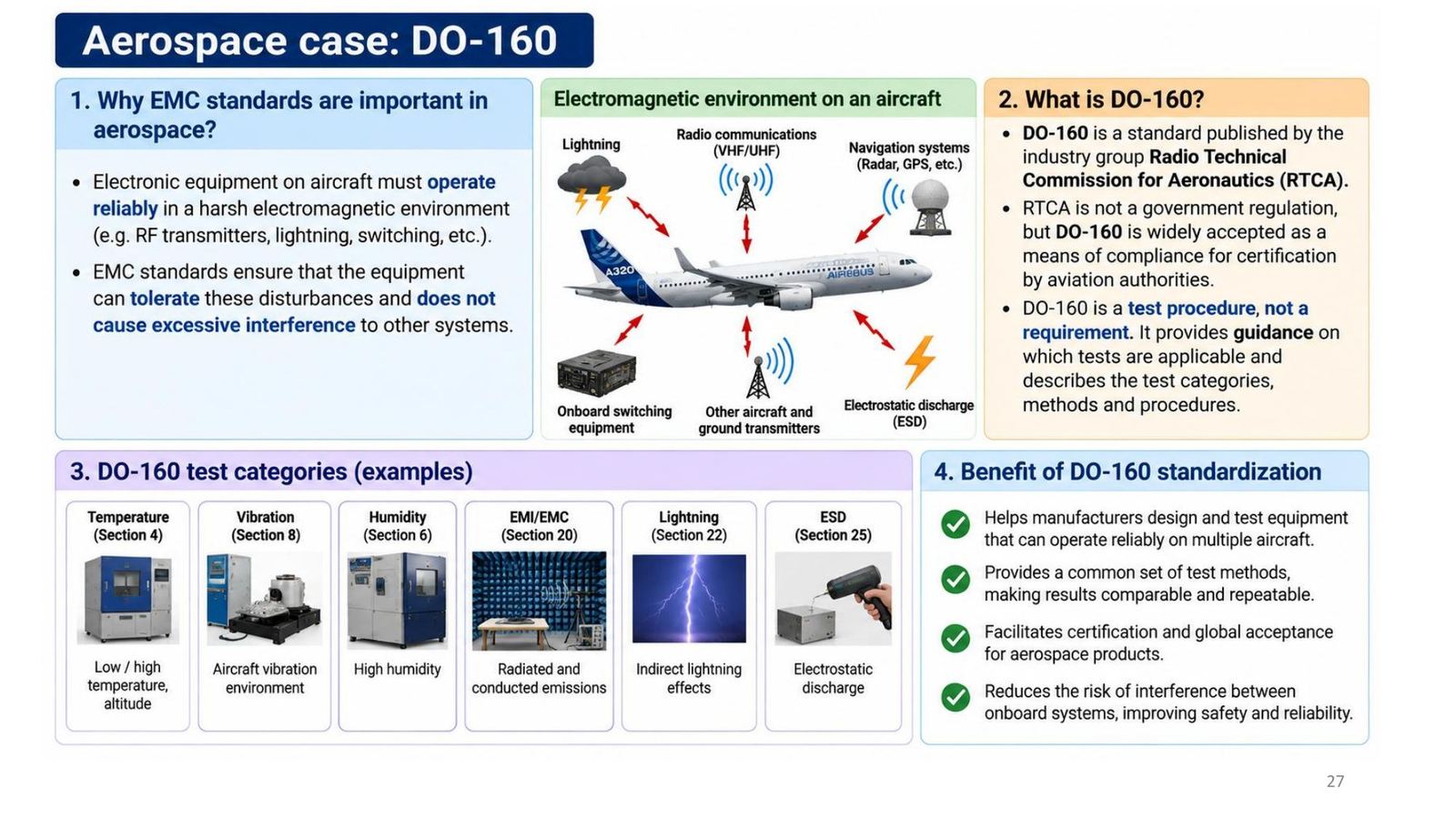
DO-160 in aerospace
DO-160 is published by the industry group Radio Technical Commission for Aeronautics (RTCA). RTCA is not a government body, but DO-160 is widely accepted by aviation authorities as a means of compliance. DO-160 is a test procedure, not a requirement: it gives guidance on which tests apply and describes test categories, methods and procedures.
| Section | Test |
|---|---|
| 4 | Temperature, altitude |
| 6 | Humidity |
| 8 | Vibration |
| 20 | EMI/EMC (conducted and radiated emission and immunity) |
| 22 | Indirect lightning effects |
| 25 | Electrostatic discharge (ESD) |
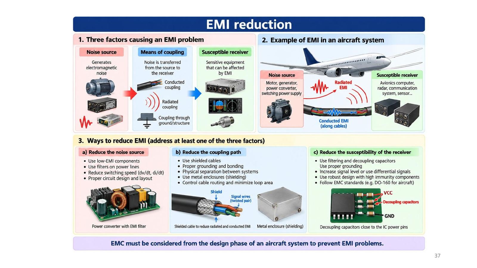
The three factors of an EMI problem
| Factor | Aircraft example | How to reduce |
|---|---|---|
| Noise source | Motors, generators, converters, switching supplies | Low-EMI components, filter power lines, slower switching (dv/dt, di/dt) |
| Coupling path | Conducted (wiring), radiated, via ground/structure | Shielded cables, grounding and bonding, separation, metal enclosures, small loop area |
| Susceptible receiver | Avionics computer, radar, communication, sensors | Filtering and decoupling, higher signal level or differential signals, robust design, follow DO-160 |
Address at least one of the three factors. EMC must be considered from the design phase.
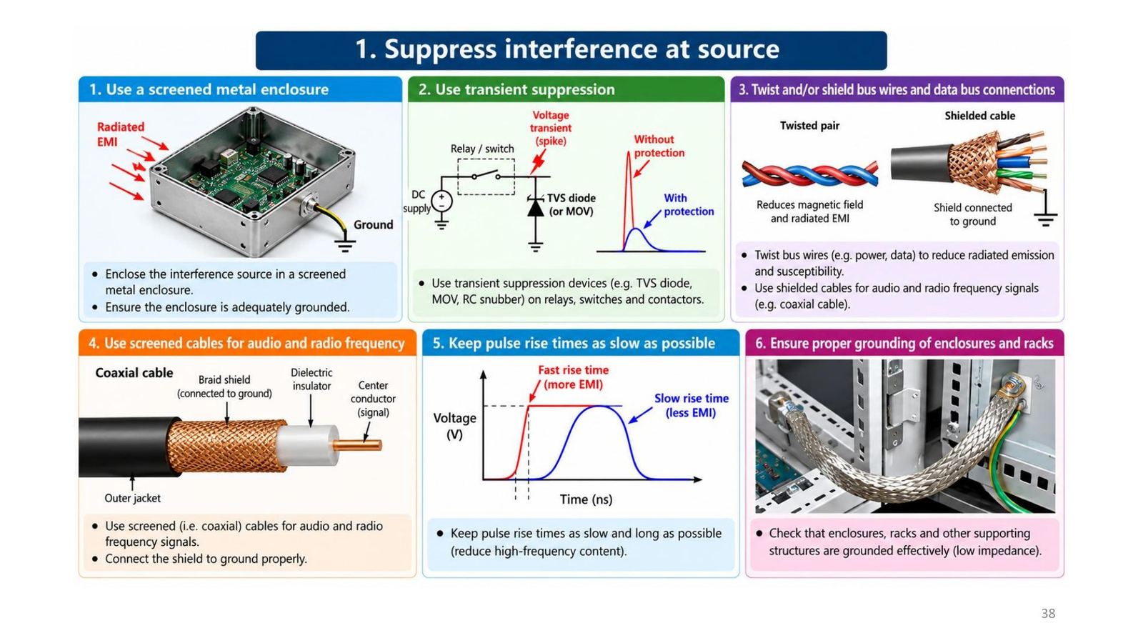
1. Suppress interference at the source
- Enclose the interference source in a screened metal enclosure and ground it adequately.
- Use transient suppression (TVS diode, MOV, RC snubber) on relays, switches and contactors.
- Twist and/or shield bus wires and data bus connections.
- Use screened (coaxial) cables for audio and radio-frequency signals, and connect the shield to ground properly.
- Keep pulse rise times as slow and long as possible (reduce high-frequency content).
- Check that enclosures, racks and supporting structures are grounded effectively (low impedance).
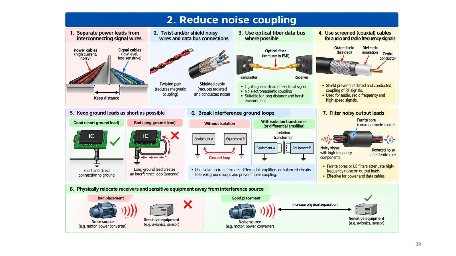
2. Reduce noise coupling and wiring practice
- Separate power wiring from signal wiring; route strategically (signals away from power).
- Twist/shield noisy wires and data buses; use optical fibre where possible (immune to EMI, Module 08).
- Keep ground leads short; break ground loops with isolation transformers, differential amplifiers or balanced circuits.
- Filter noisy output leads (ferrite cores, LC filters); relocate sensitive equipment away from the noise source.
- Keep wires short; keep shield pigtails to their designed length; do not extend equipment ground wires.
3. Increase susceptibility thresholds
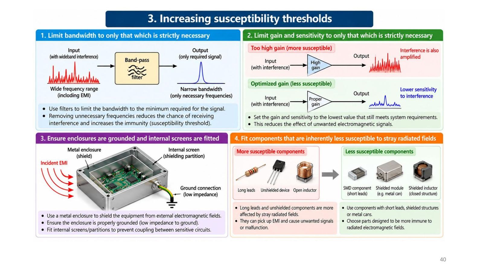
- Limit bandwidth to only what is strictly necessary (a band-pass filter removes wideband interference).
- Limit gain and sensitivity to only what is strictly necessary (excess gain also amplifies interference).
- Ensure enclosures are grounded and internal screens are fitted.
- Fit less susceptible components against stray radiated fields: short leads (SMD), shielded modules in metal cans, shielded inductors, rather than long leads, unshielded devices and open inductors.
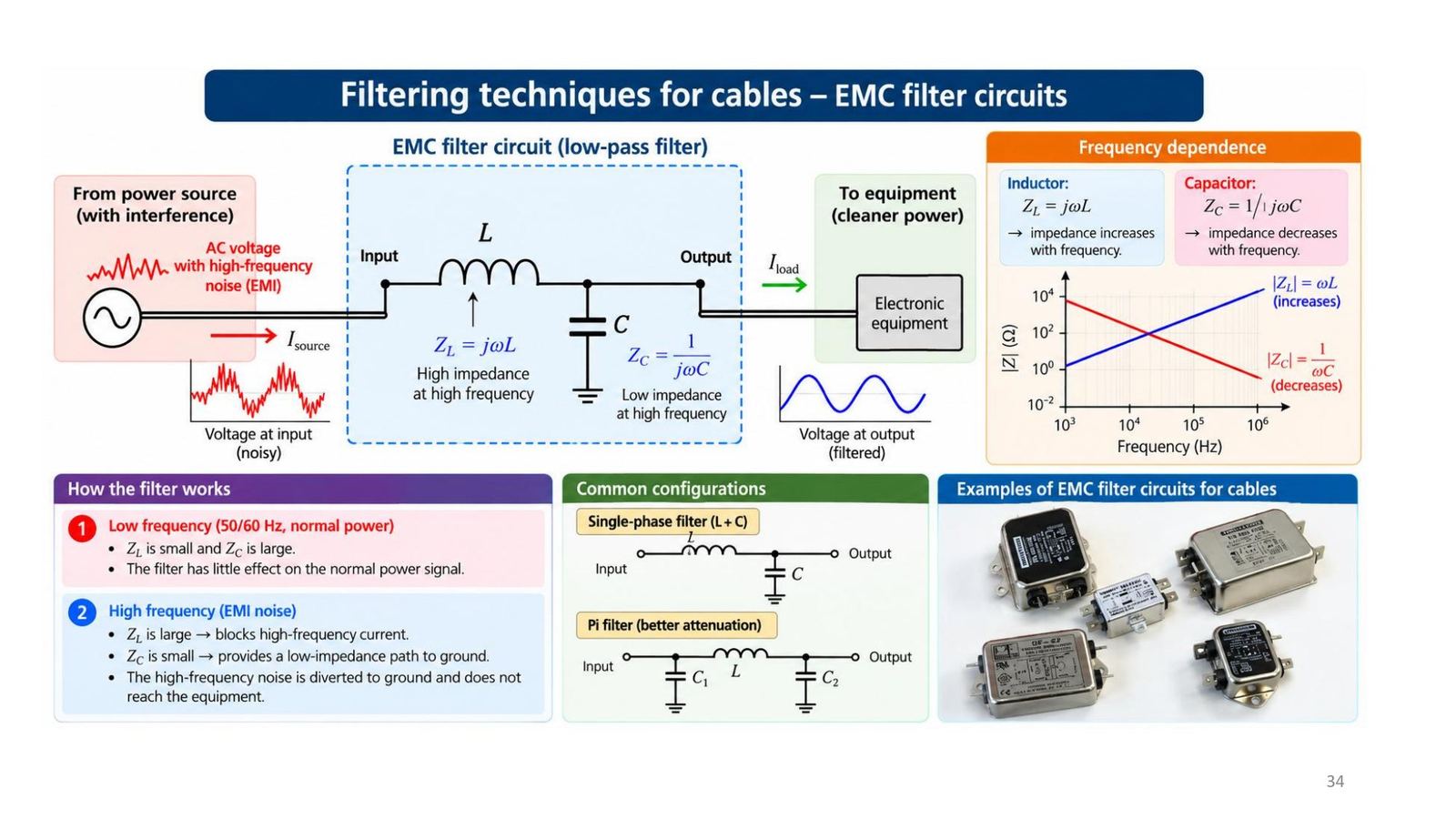
Filtering: the LC low-pass and power filters
There are many ways to filter EMI: on cables (ferrite core), at equipment inputs (LC-type EMI filter), on boards (small RC or LC). The idea is always the same: attenuate unwanted high-frequency noise while letting the useful signal pass.
A low-pass L + C filter: Z_L = jωL rises with frequency (blocks high-frequency noise), Z_C = 1/(jωC) falls with frequency (shunts high-frequency noise to ground). At 50/60 Hz Z_L is small and Z_C is large, so the filter barely affects the supply. Configurations: single-phase L + C, or the Pi filter (C, L, C) for better attenuation.
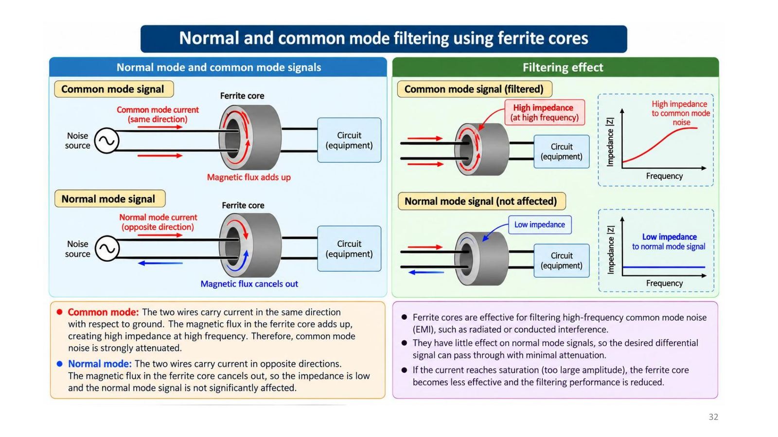
Ferrite cores: against common-mode noise
High-frequency noise current on a cable creates a magnetic field around it. A cylindrical ferrite core has high magnetic permeability μ, so it concentrates the flux; magnetic losses (hysteresis and eddy-current loss) convert energy into heat, so the cable impedance rises at high frequency and the noise current is attenuated.
| Common mode | Differential (normal) mode | |
|---|---|---|
| Current in the two wires | Same direction | Opposite directions |
| Flux in the ferrite | Adds up | Cancels out |
| Impedance | High at high frequency: noise blocked | Low: signal passes |
If the current is too large the core saturates and loses effectiveness.
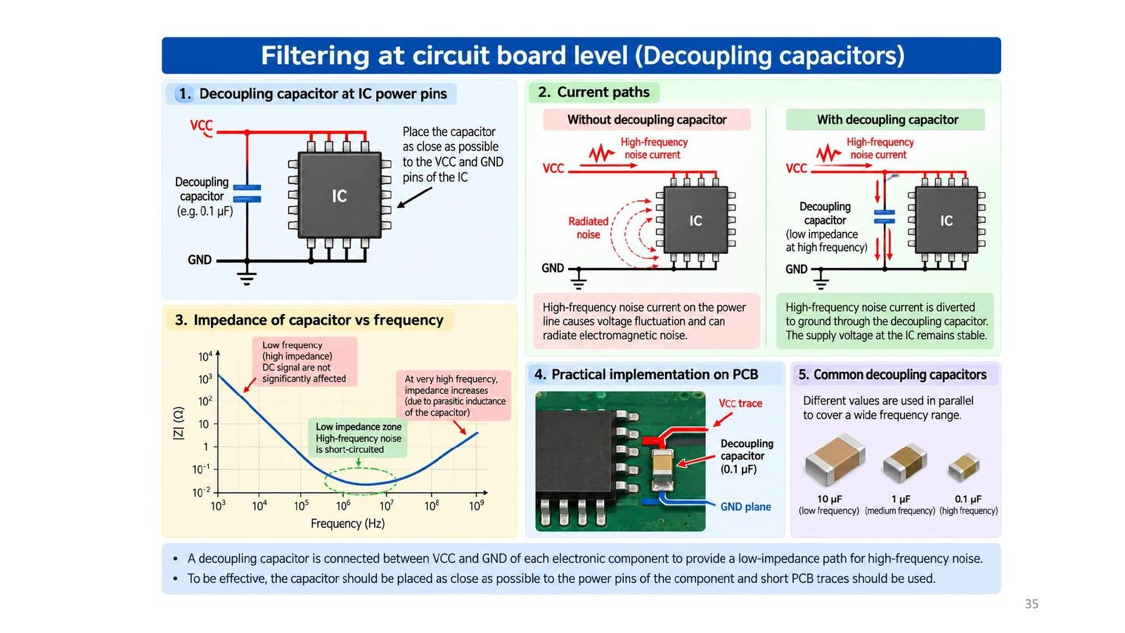
Decoupling capacitors at board level (Floyd 6-11)
A decoupling capacitor sits between VCC and ground of every component, placed as close as possible to the IC power pins with short traces, to give high-frequency noise a low-impedance path instead of running along the supply line and radiating. Several values in parallel cover a wide band: 10 µF (low), 1 µF (medium), 0.1 µF (high frequency).
Floyd 6-11 (p.364): current and voltage spikes on the VCC and ground lines from the fast switching of digital circuits; absorb them with about a 1 µF capacitor from VCC to ground for the whole board, plus small 0.022 to 0.1 µF capacitors distributed around, especially near devices switching at high rates or driving many loads (oscillators, counters, buffers, bus drivers).
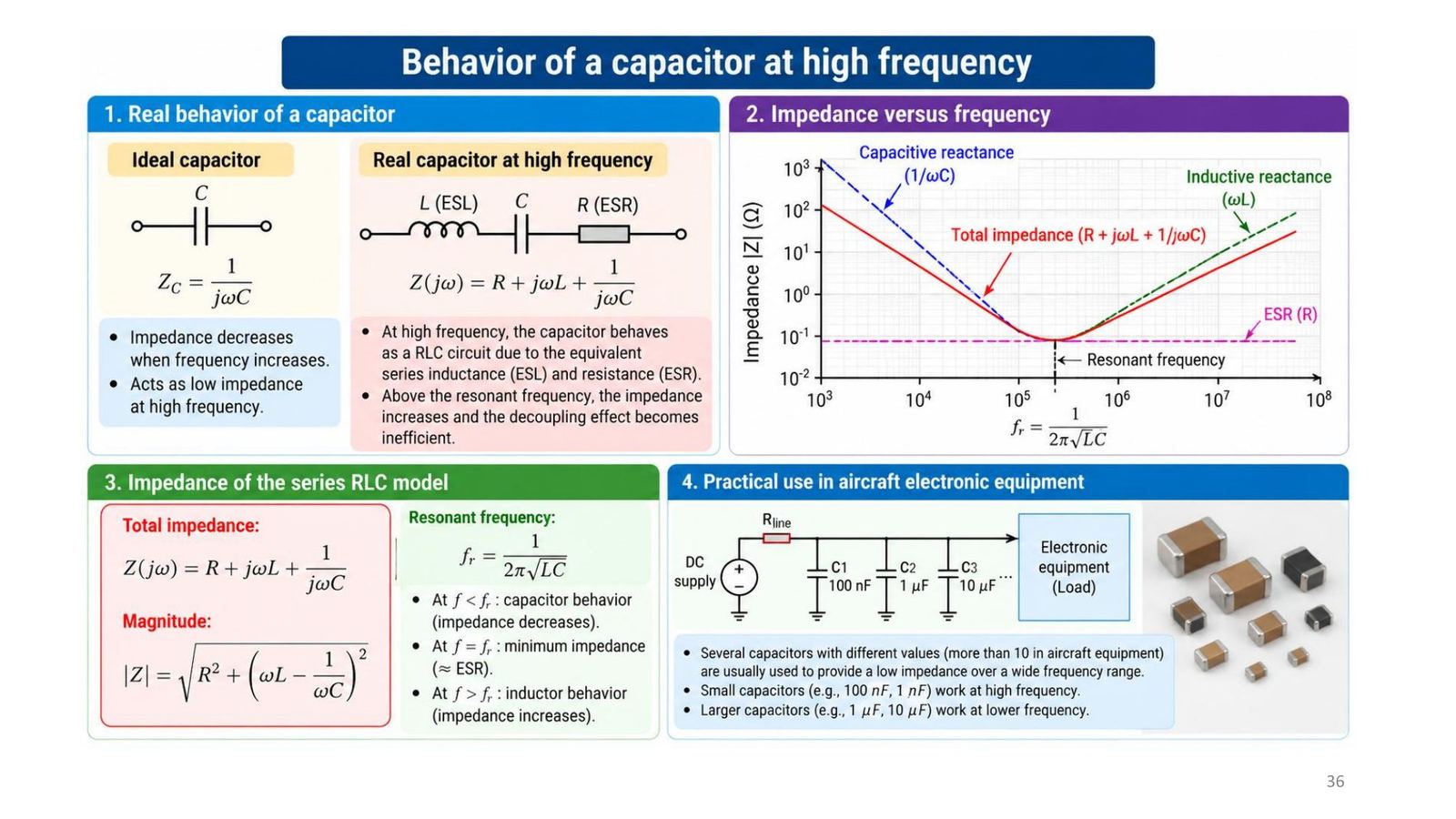
A real capacitor at high frequency: ESL, ESR and resonance
A real capacitor = R (ESR) + L (ESL) + C in series: Z = R + jωL + 1/(jωC), |Z| = √(R² + (ωL − 1/(ωC))²). Resonant frequency f_r = 1/(2π√(LC)): below f_r it behaves as a capacitor (Z falls with frequency), at f_r the impedance is minimum ≈ ESR, above f_r it becomes an inductor (Z rises) and no longer decouples well. That is why aircraft equipment uses many capacitor values (more than 10): small capacitors (100 nF, 1 nF) for high frequency, large ones (1, 10 µF) for low frequency.
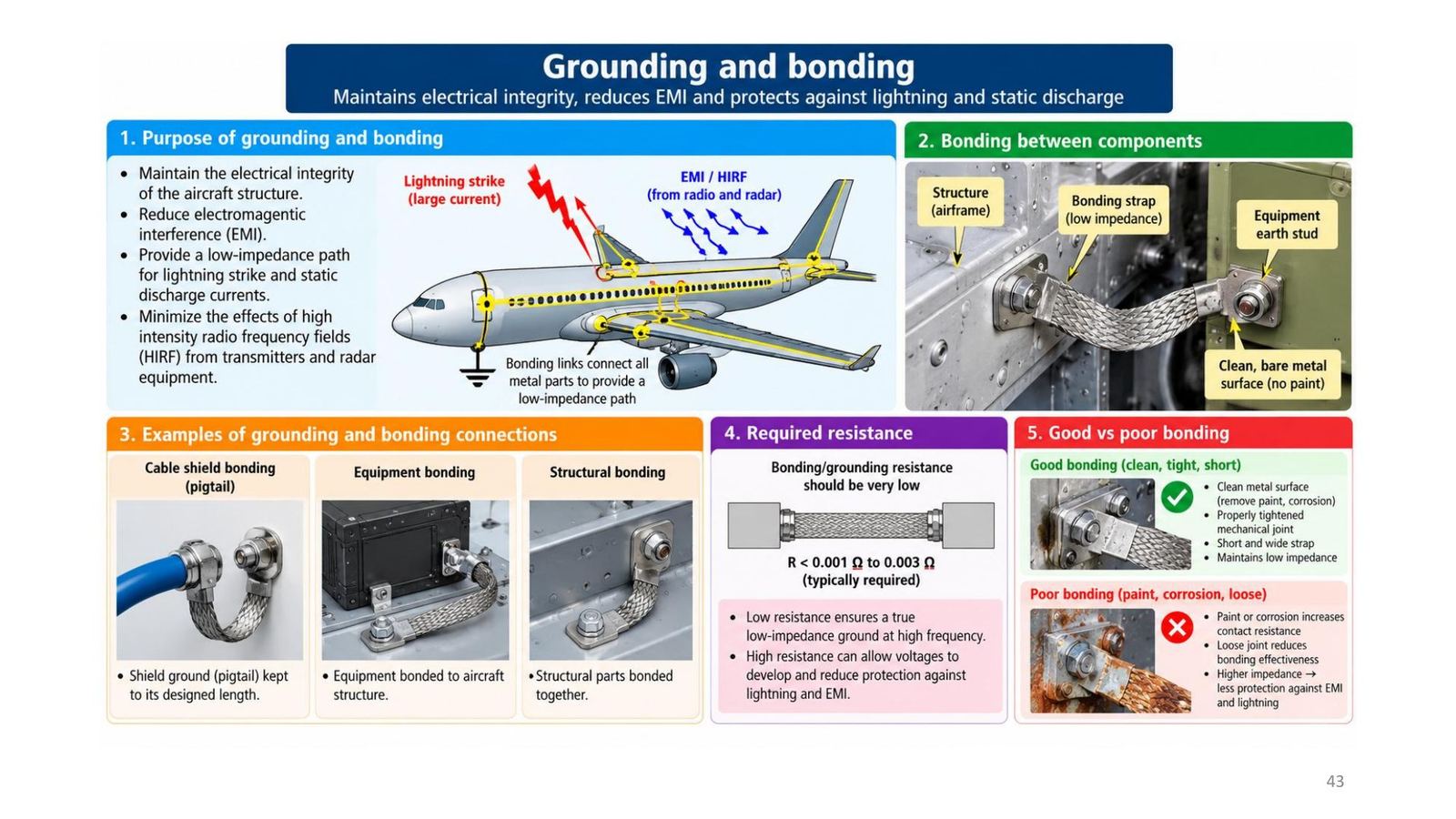
Grounding and bonding
The electrical integrity of the aircraft structure is very important to reduce EMI and protect the aircraft, passengers, crew and systems from lightning and static discharge; it also reduces the effect of high-intensity radio-frequency fields (HIRF) from high-power transmitters and radar. Use low-resistance bonding straps. Grounding and bonding resistances of less than 0.001 to 0.003 Ω are usually required.
Grounding is connecting conductive objects to a conductive structure or other return path to safely complete a normal or fault circuit; bonding is the electrical connecting of two or more conducting objects not otherwise adequately connected.
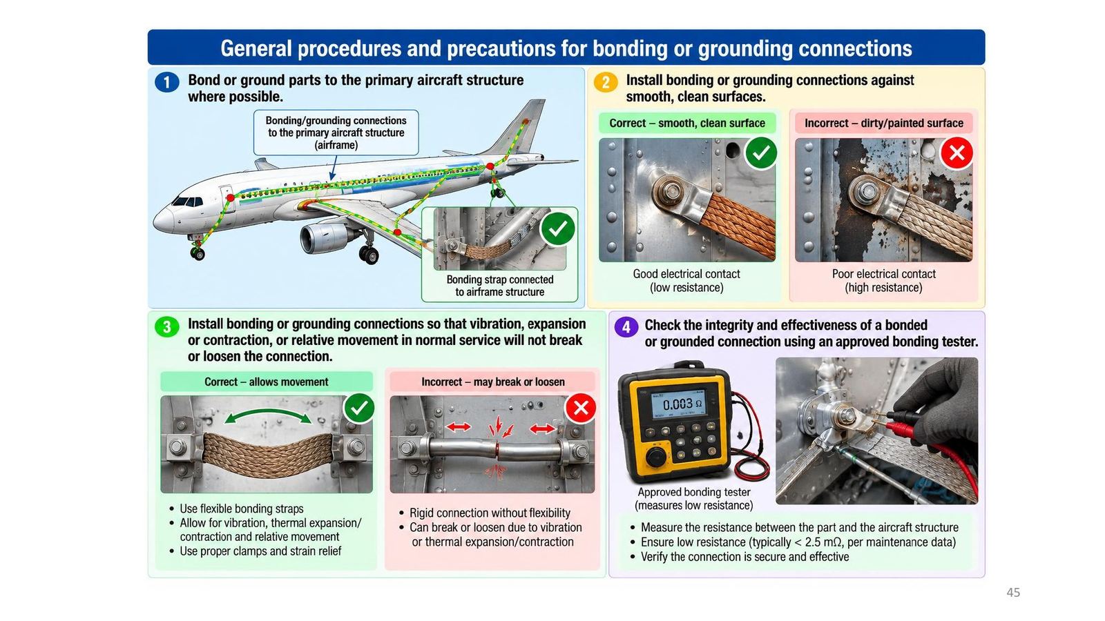
Bonding procedures and checks
- Bond or ground to the primary aircraft structure where possible; do not weaken the structure; bond parts individually if feasible.
- Install against smooth, clean surfaces (remove paint and corrosion).
- Install so that vibration, expansion or contraction, or relative movement will not break or loosen it; use flexible straps, proper clamps and strain relief.
- Check integrity and effectiveness with an approved bonding tester: measure the resistance between part and structure and compare it with the maintenance data.
🧪 Demo 1: dB, dBm and gain-chain calculator (runs in your browser)
Defaults follow the slide 20 cascade example: input 0 dBm (1 mW), +10 dB, +6 dB, minus 3 dB loss. Change the numbers to see the output level, output power and ratios.
🧪 Demo 2: a square wave is a sum of odd harmonics (Fourier)
Drag the slider to add harmonics. The odd harmonic amplitude is V/n as on slide 10 and Tooley 14.1.2.
🧪 Demo 3: a real capacitor with ESL and ESR, and its resonant frequency
Defaults: 100 nF, ESL 10 nH, ESR 50 mΩ (the module's illustrative numbers). Above the resonant frequency the capacitor becomes an inductor (slide 36).
📜 Theory and historical background
According to Tooley (section 14.2), in recent years EMC and EMI have become a very important consideration for avionic equipment designers: both the unwanted signals the equipment generates and its susceptibility to outside interference must be considered, to meet increasingly demanding standards. The lecture opens with aircraft being tested in anechoic chambers (KC-46 Pegasus, Global Hawk) and the example of Wi-Fi interfering with Honeywell Phase 3 displays on the Boeing 757; the lecture's 'Historical facts' item has only a heading and no content. The RTCA's DO-160 is not a government regulation but is widely accepted by aviation authorities as a means of showing compliance.
🔎 Case study: a 400 Hz DC supply and the parts added to meet EMC
Tooley takes a simple low-voltage DC supply (Figure 14.1) and modifies it to meet stringent EMC requirements (Figure 14.5). The added parts have four jobs: C5 to C8 give high-frequency decoupling so the regulator ICs do not oscillate; C9 and C10 remove noise on the output rails; C11, L1, L2, C12, C13 form a low-pass supply filter that removes harmonics from the diode rectifiers' switching and also blocks noise entering the equipment from the supply; finally a low-resistance ground connection links the equipment chassis to aircraft ground. All three groups of measures of the lecture are present: reduce the source (filtering harmonics), reduce coupling (grounding, screening) and raise the susceptibility threshold (decoupling). A numerical example in the same chapter: a defective switching supply raised the noise floor in the 500 kHz to 1.75 MHz band from below −110 dB to about −84 dB, i.e. 26 dB, enough to badly degrade MF reception.
⚠️ Common traps (and mismatches found in the material)
General trap: confusing 0 dBm with 0 W (0 dBm is 1 mW) and mixing the factor 10 with 20 in the dB formulas (10 for power, 20 for voltage and current). Mismatches: slide 21 (exercise 2) prints "P_out = 10000 W (10 kW)" although the calculation right next to it gives 100,000 W; the correct answer is 100 kW because 10 W × 10⁴ = 100,000 W (see Demo 1 and the notebook). Slide 43 requires a bonding resistance of 0.001 to 0.003 Ω, whereas slide 45 says "typically below 2.5 mΩ" and the tester picture there reads 0.003 Ω, i.e. 3 mΩ, above 2.5 mΩ and therefore failing by that slide's own rule; Tooley says below 0.001 to 0.003 Ω and quiz question 6 says below 0.005 Ω, so the sources use different thresholds and the manufacturer's maintenance data must be followed. Tooley (Figure 14.14) says the noise floor rose by 26 dB "or 50 times"; 26 dB is about 20 times in amplitude (about 400 times in power), not 50. Slide 10 and Tooley 14.1.2 write the square wave as V sin ωt + (V/3) sin 3ωt + …; that is a simplified scaled form, since the fundamental of a square wave of amplitude V is really 4V/π, so read V there as the fundamental amplitude, not the square-wave amplitude. Slide 1 misspells "Dndergoes" in the Global Hawk caption, slide 16 repeats slide 15, and the slide 2 heading "Historical facts" has no content. On the Floyd side: Floyd has no EMC chapter; it mentions EMI only at cable level (twisted pairs reduce crosstalk, shielded STP resists EMI), board-level decoupling capacitors, and the noise margin of logic families.
📓 Companion Python notebook
Companion notebook: recomputes every dB, dBm and cascade number in the lecture (slides 14 to 21), catches the 10 kW versus 100 kW error, verifies the square-wave Fourier series, computes f_r and the impedance of a real capacitor, the numbers in Tooley's spectrum-analyser examples, the noise margins of Floyd chapter 15 Problem 3, and re-runs the quiz questions that can be computed.
✅ Self-check quiz
Book 1: Mike Tooley, Aircraft Digital Electronic and Computer Systems (end-of-chapter MCQs, independently recomputed to verify each answer)
Book 2: Thomas Floyd, Digital Fundamentals (True/False Quiz + Self-Test, cross-checked against the book’s own printed answer key)
Additional practice questions (AI-authored in the same style, answers self-verified by computation)
✍️ Free-response questions (source: Floyd, Digital Fundamentals)
Floyd Digital Fundamentals 11th ed.: Ch.13 Problem 3 (p.793, answer A-27) and Ch.15 Problem 3 (p.887, answer printed on A-28). Tooley ch.14 has only Test Your Understanding without printed answers, so they are not presented as problems with real answers; they are solved in the slides and notebook.
Floyd has no EMC exercises; the two nearest odd problems (crosstalk and noise margin) have printed answers and are included with the real answer images. The lecture's dB exercises (slides 17, 19, 21) are solved in the slides and notebook.
13-3. What is crosstalk? How can it be minimized?

Matches Floyd 13-1 (p.741) and the Section Checkup: the twisted wires cross at nearly 90° so the electromagnetic fields cancel. This is also the module's twisting measure (slides 29, 38).
Floyd Ch.13 · Problem 3
👁️ Show the book's original answer

15-3. A TTL gate has the following actual voltage level values: VIH(min) = 2.25 V, VIL(max) = 0.65 V. Assuming it is being driven by a gate with VOH(min) = 2.4 V and VOL(max) = 0.4 V, what are the HIGH- and LOW-level noise margins?

Own calculation by Equations 15-1 and 15-2: V_NH = 2.4 − 2.25 = 0.15 V; V_NL = 0.65 − 0.4 = 0.25 V, matching the printed answer (A-28).
Floyd Ch.15 · Problem 3
👁️ Show the book's original answer
