Introduction: why transform methods

Introduction: why transform methods

• Explain the "change domain, then solve" idea behind every linear transform.
• State the two conditions (linearity, time invariance) under which a harmonic input gives a harmonic output at the same frequency.
• Read a spectrum from an FFT, know leakage and phase, and check it with a direct sum.
• Recognise the symbols \Pi, \delta, \text{III} and the asterisk * used throughout the book.
• Know where the two source books of this course (Bracewell and Barkat) meet.

Use the buttons, the dots or the ← → keys to move between slides.

Change domain, solve, change back

Bracewell opens by saying that linear transforms named for Fourier and Laplace are techniques for solving problems in linear systems. The transform is a mathematical or physical tool that alters the problem into one that can be solved (p. 1).

1. Transform the problem to the frequency domain.
2. Solve there, usually with just multiplication and division.
3. Invert to get the answer in the original domain.

The Fourier transform pair

• f(x)original function of the variable x (time or space)
• F(s)the Fourier transform, a function of frequency s
• sfrequency: cycles per unit of x

Numerical example: convolution becomes multiplication

Bracewell computes the serial product of \{2,2,3,3,4\} and \{1,1,2\} by hand on p. 32. The notebook does it two ways: the direct sum, and multiplying two FFTs then inverting. Both give the sequence 2 4 9 10 13 10 8.

Fourier before Laplace

Going through Fourier first means that when the more general Laplace transform arrives later, many properties are already familiar. Only the new and essential question remains: the strip of convergence in the complex plane (p. 1).

One theorem, many physical embodiments

Bracewell notes that a concept familiar in one branch often appears in a different guise in another: the phase-contrast microscope is reminiscent of the circuit that detects frequency modulation, and both are explained by transforms along the same lines. A statistics problem may yield to an approach familiar from cascaded amplifiers (p. 1).

It is also why this course pairs Bracewell with Barkat: the same convolution appears in signal filtering and in the distribution of a sum of random variables.

Reversing the traditional order

In traditional courses the Fourier transform shows up in the last lecture of a long course on Fourier series. Reverse the order and the series falls into place as an extreme case within transform theory, and its mathematical difficulties are tied to its non-physical extreme nature (p. 2).

Module 13 rebuilds the Fourier series from multiplication by the impulse train \text{III}.

Same information in both domains: energy conservation

For a 1000-point test signal, the sum of squares in time is 123.1328 and \frac1N\sum|X_k|^2 in frequency is 123.1328. The two are equal (Rayleigh's theorem, module 6).

Self-check, part 1

• Why does the sum of the terms of a convolution equal the product of the two sums? (Hint: set s=0 in the transform of the convolution.)
• If a signal has time-domain energy 123.1328, what must its frequency-domain energy be?
• Why does Bracewell call the Fourier series an "extreme" case?

Hints: F(0)=\int f, so the transform of the convolution at s=0 equals F(0)G(0); the second answer is exactly 123.1328; the third: because an infinite periodic signal has no ordinary transform (module 2).

Three sinusoids: reading the spectrum from an FFT

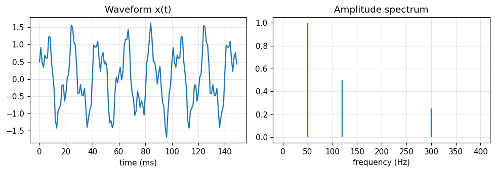
The test signal has 1.0 at 50 Hz, 0.5 at 120 Hz and 0.25 at 300 Hz. The FFT recovers the amplitudes 1, 0.5 and 0.25.

The spectrum is something you can measure

An oscilloscope shows an electrical waveform, a spectrum analyzer shows electrical or optical spectra, and the ear hears spectra (Bracewell, p. 1).

• Waveform: x(t), measured with an oscilloscope.
• Spectrum: X(f), measured with a spectrum analyzer or by ear.
• The two are Fourier transforms of each other, so they carry the same information.

Two ways to compute a spectrum, one answer

Method A uses the FFT. Method B sums directly from the definition X_k=\sum_n x_ne^{-i2\pi kn/N} (Bracewell's "slow Fourier transform", chapter 7). They differ by at most 2.4e-14, i.e. they agree to rounding error.

• Nnumber of samples
• X_kthe k-th DFT coefficient
• A_kamplitude of the sinusoid at frequency k\,f_s/N

Frequency resolution

Observing 1 second at 1000 Hz sampling gives 1000 samples and frequency bins spaced f_s/N=1 Hz apart. To separate two lines 0.5 Hz apart you must observe for at least 2 seconds.

• Tobservation time
• f_ssampling rate

Leakage: when the frequency falls between two bins

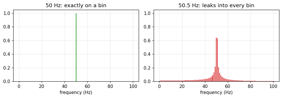
A 50.5 Hz wave analysed over 1 second falls on no bin. The amplitude at bin 50 is only 0.6397 (instead of 1), the prediction |\text{sinc}(0.5)| is 0.6366, and even at bin 80 there is still 0.0085.

Phase: how sin and cos differ

The amplitude spectrum does not tell \sin from \cos; the phase does. The FFT gives phase -90 degrees at bin 50 for the \sin and 0 degrees at bin 120 for the \cos.

Frequency s is cycles per unit, not rad/s

The book keeps 2\pi in the exponent so s is the number of cycles per unit of x (pp. 6, 18). If another text uses \omega, convert with \omega=2\pi s.

The spectrum of a sum is the sum of the spectra

The Fourier transform is linear: \mathcal F\{x_1+x_2\}=\mathcal F\{x_1\}+\mathcal F\{x_2\}. The notebook checks it with two signals; the largest deviation is 6.2e-14, of the order of rounding error.

Harmonic response to harmonic stimulus

The response of a system to harmonic input is itself harmonic, at the same frequency, under two conditions: linearity and time invariance (Bracewell, p. 3). That is why an amplifier is specified by its frequency response.

Two conditions merged into one: convolution

The two conditions can be restated as one: the response is relatable to the stimulus by convolution (p. 3).

• x(t)stimulus (input signal)
• h(t)impulse response of the system
• y(t)response (output signal)

Impulse response of a first-order low-pass filter

The filter y[n]=a\,y[n-1]+(1-a)\,x[n] with a=0.9 has impulse response h[n]=(1-a)a^n. Direct convolution with h and the lfilter function give the same answer (largest deviation 8.2e-15), and the sum of h is 1, i.e. unit DC gain.

Test with a 50 Hz wave

Input at 50 Hz, sampled at 1000 Hz. The output frequency is 50 Hz. The measured gain is 0.3193, the theoretical gain 0.3193. The measured phase is -62.62 degrees, the theoretical -62.62 degrees (negative means the output lags).

Frequency response at several frequencies

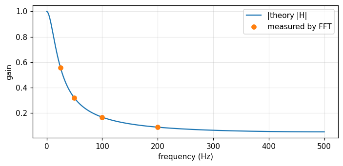
Measured by FFT at 25, 50, 100 and 200 Hz, the gains are 0.5576, 0.3193, 0.1681 and 0.0893, matching the theoretical curve. A low-pass filter: the higher the frequency, the smaller the amplitude.

When the conditions fail, new frequencies appear

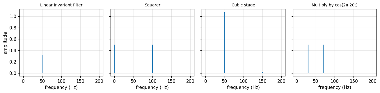
A 50 Hz wave through a squarer (nonlinear): DC component 0.5, a 100 Hz component of amplitude 0.5, and only 0 left at 50 Hz. Multiplied by \cos(2\pi\,20t) (linear but time-varying): two components at 30 Hz and 70 Hz with amplitudes 0.5 and 0.5.

Harmonic distortion of an amplifier with a cubic term

The stage y=x+0.1x^3 driven at 50 Hz gives a fundamental 1.075 and a third harmonic at 150 Hz of 0.025. The total harmonic distortion \text{THD}=A_3/A_1 is 2.33%.

Three traps with the word "linear"

• Linearity alone is not enough: the \cos(2\pi\,20t) multiplier is linear but time-varying, so it creates new frequencies.
• Time invariance often survives when linearity fails, but space invariance is far less common: bridge deflection is not split into spatial sinusoids (p. 3).
• When linearity fails (nonlinear servomechanism), harmonic analysis must be reconsidered (p. 3).

Four symbols used throughout

The rectangle is a "gate" function

The rectangular pulse is at least as simple as a Gaussian pulse, so Bracewell gives it its own name \Pi(x). The electronics term "gate function" suggests the use: multiply a waveform by \Pi(t) to open a valve for one segment (p. 2).

Example: the integral \int\Pi(x)\cos(\pi x)\,dx equals 0.6366, exactly 2/\pi.

The asterisk replaces an integral with a dummy variable

Writing \Pi*f or \Pi(x)*f(x) for \int_{x-1/2}^{x+1/2}f(u)\,du is a small step, but the dummy variable and limits vanish and the running-mean character shows (p. 3). For f(u)=e^{-u^2} at x=0: numerical integration gives 0.9226, the formula \sqrt\pi\,\text{erf}(1/2) gives 0.9226.

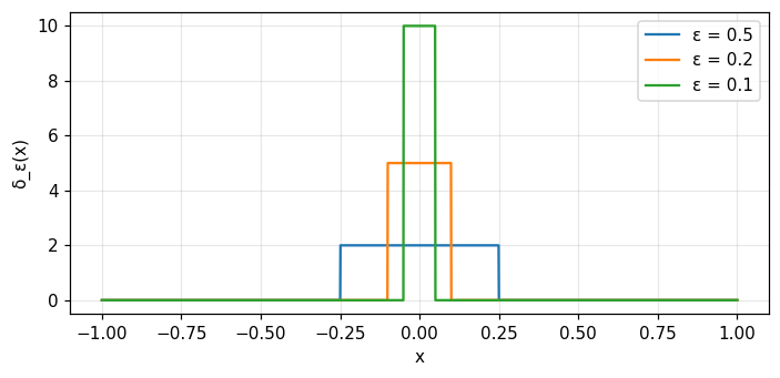
The impulse is a limit, not a function

The term "impulse symbol" reminds us that \delta(x) is not a function. An expression containing it has meaning as the limit of a sequence of pulses (not impulses) growing narrower and taller, and that limit often exists (p. 4).

• \varepsilonpulse width, made to approach 0

Numerical test: the impulse "sifts" the value at the origin

With f=\cos x, the integral \int f\,\delta_\varepsilon\,dx approaches f(0)=1 as \varepsilon shrinks:

This is the "sifting" property developed in chapter 5.

Why it is called an impulse "symbol"

In physics, Green's functions and impulse responses can often be produced or observed within the resolving power of the equipment, while impulses themselves are fictitious. Familiar examples are the moment produced by a point mass on a beam and the electric field of a point charge (p. 4).

The impulse train \text{III} (shah): sampling and periodicity

Shah is defined as \text{III}(x)=\sum_n\delta(x-n). Regular sampling (tabulation) is multiplication by shah, and periodic functions are convolutions with shah. Since shah is its own Fourier transform, it is twice as useful as might be expected (pp. 2 to 3).

Generalized functions: chapters 5 and 6

Bracewell prefers the presentation through "generalized functions" following Temple and Lighthill (chapters 5 and 6). It retains both rigor and the direct procedures of manipulating \delta that have been so successful (p. 4).

The two source books

26 modules: 4 shared, 15 Bracewell only, 7 Barkat only

Each chapter is a module. Four pairs of chapters on the same topic are merged into one longer module (about 60 slides instead of 40):

Five parts, A to E

Thinking in transforms is not computing them

Transform methods do not necessarily involve taking transforms numerically. Some of the best methods for linear problems do not apply the transform to the data at all, though their basis is clarified by appeal to the transform domain (p. 3).

For numerical work one normally prefers the answer as the convolution of two functions rather than as a Fourier transform (p. 3). That is why module 3 comes right before the theorems.

This course's routine: two independent methods

• Every number on the page is printed by the notebook, never typed by hand.
• Each number is computed by at least two independent methods (for example FFT and direct sum, numerical integral and closed form), and the notebook stops if they disagree.
• The Vietnamese and English editions use the same code and must print exactly the same numbers.

Examples from this very module: FFT and direct sum differ by 2.4e-14; the convolution filter and lfilter differ by 8.2e-15.

How to study a module

1. Read the objectives and step through the slides in 5 parts. Use the slide list to jump.
2. Read the history, the case study and the formula sheet.
3. Open the notebook, run each cell, read the "Real output" note after it, then change the parameters yourself.
4. Take the quiz, read the explanations of wrong answers, and return to the matching slides.

Notation and conventions of the book

Self-check, part 5

• Which chapters of Bracewell and Barkat are merged to teach random processes and noise?
• Why does "thinking in transforms" not mean you must always compute an FFT?
• If the FFT and the direct sum disagree by a lot, what do you do before trusting the number?

Hints: chapter 17 and chapter 3; because the answer sometimes comes out directly as a convolution; investigate the cause to the end.

Takeaways

• A transform is a tool: change domain, solve, change back.
• A waveform and its spectrum carry the same information (energy is conserved), and both are measurable.
• Reading a spectrum needs care with the resolution f_s/N, leakage and phase.
• A harmonic input gives a harmonic output at the same frequency when the system is linear and invariant; the response is then a convolution.
• \delta(x) is a limit of pulse sequences, not an ordinary function.
• The course has 26 modules pairing two books, and every number is checked by two methods.

References

R. N. Bracewell, The Fourier Transform and Its Applications, 3rd ed., McGraw-Hill, 2000, chapter 1 (pp. 1 to 4), chapter 2 (pp. 5 to 8), chapter 3 (pp. 24, 30 to 34) and epigraph.
M. Barkat, Signal Detection and Estimation, 2nd ed., Artech House, 2005, section 1.3.1 (step and impulse functions) and the table of contents of chapters 1 to 12.
The content was written with AI assistance (Claude) and then checked. Every number is produced by a Jupyter notebook and cross-checked by two independent methods; page citations come from the OCR text of the two source books. Mistakes may remain, so please report them.
R. N. Bracewell, The Fourier Transform and Its Applications, 3rd ed., McGraw-Hill, 2000.
M. Barkat, Signal Detection and Estimation, 2nd ed., Artech House, 2005.
This site only summarises, explains and checks numbers; please read the original books through a library or the publisher.
Contribute
Report errors, suggest modules or translations in the GitHub repository, and fork or clone it for your own study. Please credit the source when sharing.