Convolution, serial products and correlation

Convolution, serial products and correlation

• Define convolution and picture it four ways: area, smoothing, superposition, folding.
• Compute the convolution of truncated exponentials and of number sequences by hand, checked by the sum of terms.
• Invert a serial product (serial division), use the table of reciprocal sequences and write convolution as a matrix.
• Compute convolution by machine and know when an FFT wraps around.
• Use autocorrelation, cross correlation, triple correlation and the energy spectrum, and know what information they discard.

Use the buttons, the dots or the ← → keys to move between slides.

One concept, many names

Convolution occurs widely under many aliases: Faltung (German), composition product, superposition integral, Duhamel integral, Borel's theorem, (weighted) running mean, cross-correlation function, smoothing, blurring, scanning, smearing (Bracewell, p. 24).

Definition

The convolution of f(x) and g(x) is itself a function of x, called h(x) (p. 24).

• udummy variable of integration
• g(x-u)g reversed and shifted to x

A functional: it needs f over a whole range

Following Volterra, h is a functional of f. To calculate h(x_1) we need f over a whole range of x, whereas a function of the function f at x=x_1 needs only f(x_1) (p. 25). That is why convolution describes the "memory" of a system.

View 1: the area of the product f(u)g(x-u)

In Fig. 3.1 the product f(u)g(x-u) is shaded and the ordinate h(x) equals the shaded area (p. 25). Numerical example: f=\Pi and g=e^{-u}H(u); at x=1 the overlap area is e^{-1/2}-e^{-3/2} = 0.3834 (numerical integral and closed form agree).

View 2: smoothing

Compared with f, the function h=f*g is smoother in detail, more spread out and has less total variation (Fig. 3.2, p. 25). Example: a \pm1 series that flips sign constantly has total variation 48; after a 5-point running mean it has 11.6.

Views 3 and 4: superposition and folding

View 3: resolve f into infinitesimal columns, each "melted out" into a heap shaped like g centred at the column, and h(x) is the sum of contributions at x (Fig. 3.3). View 4: fold g(u) about the line u=x/2; the area under the product is h(x) (Fig. 3.4) (pp. 25 to 26).

Algebra: commutative, associative, distributive

Because g is reversed before multiplying, convolution is commutative. It is also associative (when the integrals exist) and distributive over addition, so the asterisks behave like multiplication signs in formal manipulation (pp. 26 to 27). The notebook checks all three on random sequences: 3 of 3 hold.

Physical meaning: every observation is a convolution

Convolution describes the action of an observing instrument when it takes a weighted mean of some physical quantity over a narrow range of a variable. When the weighting function does not change with position, the observed quantity is a convolution rather than the desired quantity itself. All physical observations are limited by the resolving power of instruments, and for this reason alone convolution is ubiquitous (p. 24). Its appearance is coterminous with linearity plus invariance, and with harmonic response to harmonic stimulus.

Self-check, part 1

• Why is convolution commutative even though g is reversed and f is not?
• Why is h(x) called a functional of f?
• When is an observed image the convolution of the object with the instrument?

Hints: substitute u\to x-u; it needs f over a range; when the weighting function does not change with position.

Convolution of two truncated exponentials

Let E(x)=e^{-x}H(x). For two different positive decay constants \alpha,\beta, Bracewell computes (p. 27):

• \alpha,\betadecay constants

Numbers: a radioactive decay chain

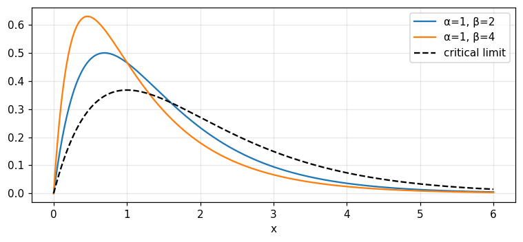
The result is the difference of two truncated exponentials with the same amplitude. It describes the concentration of an isotope decaying with constant \alpha while replenished as the decay product of a parent isotope decaying with constant \beta. With \alpha=1,\beta=2 at x=1: numerical integration and the formula give 0.4651. As x\to\infty only the more slowly decaying term survives (p. 28).

The limit \beta\to\alpha: the critically damped resonator

Taking \beta-\alpha\to0 gives \alpha E(\alpha x)*\alpha E(\alpha x)=\alpha^2xE(\alpha x). This function describes the response of a critically damped resonator, such as a dead-beat galvanometer, to an impulsive disturbance (p. 28). With \alpha=1 at x=2: 0.2707.

Two opposed tails

\alpha E(-\alpha x)*\beta E(\beta x) gives a function peaked at the origin dying away with constant \alpha to the left and \beta to the right (pp. 28 to 29). With \alpha=1,\beta=2: at x=-1 it is 0.2453, at x=+1 it is 0.0902, so the right side falls faster.

Graphical construction: the sliding paper

To check a calculation, plot one function backward on a movable piece of paper and slide it along the abscissa. To the left, the product is zero. Then the integral starts to be nonzero, increases nearly linearly, reaches a maximum and dies away. This shows at once the opposed tails, the absence of a zero stretch and the jump in slope at the origin (pp. 29 to 30). Experts do this in their heads.

Repeated convolution of the rectangle

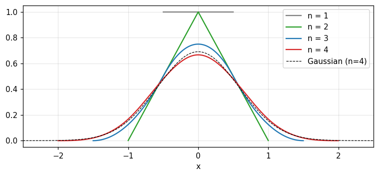
\Pi*\Pi=\Lambda (a triangle), then \Pi*\Pi*\Pi is a piecewise parabola. The notebook repeats the convolution on a fine grid: at x=0 the value is 0.75 (exactly 3/4) and at x=1 it is 0.125 (exactly 1/8). Each convolution makes the shape smoother and more Gaussian.

Rules for area and variance

For unit-area functions, convolution multiplies areas (so the area stays 1) and adds variances. For example e^{-x}H(x) (variance 1) convolved with \Pi (variance 1/12) gives variance 1.0833 and area 1. Repeating \Pi n times has variance n/12; the largest deviation from a Gaussian of the same variance is 0.0243 for n=4 and 0.0092 for n=8.

Self-check, part 2

• Which function does the result approach as \beta\to\alpha?
• Which side of \alpha E(-\alpha x)*\beta E(\beta x) decays faster if \beta>\alpha?
• What is the variance of the convolution of three rectangles?

Hints: \alpha^2xE(\alpha x); the right side; 3/12=1/4.

Multiplying polynomials is a serial product

The product of two polynomials a_0+a_1x+\dots and b_0+b_1x+\dots has coefficients c_0=a_0b_0, c_1=a_0b_1+a_1b_0, c_2=a_0b_2+a_1b_1+a_2b_0, ... These are exactly the sums of discrete convolution (Bracewell, p. 30). The notebook compares polymul with convolve and finds them equal.

Length and sum: two quick checks

The serial product is longer than either component: the number of terms is the sum of the lengths minus one. The sum of the terms equals the product of the sums, a very valuable numerical check. If one sequence sums to unity the product sums to the same as the other (p. 32). Example: a 7-term sequence with a 4-term one gives 10 terms.

Semi-infinite and two-sided sequences

A semi-infinite sequence such as \{1,1\}*\{1,2,3,\dots\}=\{1,3,5,7,\dots\} still gives a valid serial product since each term sums only finitely many terms. But if two sequences run on in opposite directions each term is an infinite sum that may not exist. Two-sided sequences need the origin stated explicitly, for example by an arrow (pp. 32 to 33).

Special sequences

The sequence \{\dots0,0,1,0,0,\dots\} plays the role of the impulse: convolving with it changes nothing. \{1,-1\} takes the first difference. \frac1n\{1,\dots,1\} (n terms) is a running mean; for example a weekly mean of daily values is \frac17\{1,1,1,1,1,1,1\}. \{1,1,1,\dots\} gives running sums (p. 33).

Numerical test: running sums and differences invert each other

For the sequence \{3,1,4,1,5,9,2,6\} the running sum ends at 31, and taking differences with \{1,-1\}* returns exactly the original. This is the relation \{1,1,1,\dots\}*\{1,-1\}=\{1,0,0,\dots\} (p. 34): the two sequences are reciprocal, like integration and differentiation.

Reciprocal sequences

The reciprocal sequence \{f\}^{-1} of \{f\} satisfies \{f\}^{-1}*\{f\}=\{1,0,0,\dots\}. If \{f\}*\{g\}=\{h\} and \{f\}, \{h\} are known, then \{g\}=\{f\}^{-1}*\{h\}. For example \{1,2,3,4,\dots\} and \{1,-2,1\} are a reciprocal pair (p. 34). The notebook checks: 2 of 2 pairs hold.

Serial division: finding the other factor

To solve \{1,1\}*\{g\}=\{1,3,3,1\} one can do long division of polynomials or use Bracewell's method: g_0=h_0/f_0, then each next term is h_k minus the sum of the known products, divided by f_0 (pp. 34 to 36). Both give \{g\} = (1 2 1).

Table 3.1: sequences and their inverses

Bracewell lists common pairs (p. 37); the notebook checks 6 of the first 6 pairs by multiplying and looking for {1, 0, 0, ...}.

Matrix form and time-varying systems

The serial product can be written as a square matrix (each row the sequence \{f\} reversed and shifted one step) multiplying a column vector. That matrix is a Toeplitz matrix. The notation sacrifices commutativity but generalises: if the rows change we get the general linear transformation, not shift-invariant. For a time-varying system (such as motor-driven potentiometers) the response is no longer a convolution and "harmonic response to harmonic excitation" also breaks down (pp. 37 to 39). The notebook checks: the Toeplitz matrix product and convolve agree (yes).

The direct code

Bracewell gives a short code for direct convolution: for sequences of lengths l_f and l_g the convolution has length l_h=l_f+l_g-1, and each h(I) sums the products f(J)g(K) with K=I-J+1 (p. 40). In applications to filtering long data sets this code will usually run faster than a transform method written in the same language (p. 40).

Numerical test: hand code versus convolve

The notebook translates the code to Python and compares it with numpy.convolve on two pairs of random sequences (lengths 200 and 37, then 5 and 5): the results agree to rounding error, largest deviation 5.3e-15.

Three length modes

For sequences of length 10 and 4: full mode (every overlapping position) gives 13 terms, same gives 10 (the length of the longer) and valid (only where they overlap completely) gives 7. When smoothing data, remember that the edges are affected.

Counting multiplications: direct versus FFT

Direct convolution needs l_fl_g multiplications. Through the FFT it needs three transforms of length N\ge l_f+l_g-1, of order 3N\log_2N operations (an order-of-magnitude estimate). With l_f=10^5 and a short filter l_g=32: direct 3,200,000, FFT about 6,684,672, the same order. With a long filter l_g=2000: direct 200,000,000, the FFT still about 6,684,672, clearly faster.

The wrap-around trap

Multiplying two FFTs of length N smaller than l_f+l_g-1 gives a circular convolution, not a linear one: the tail wraps around to the start (chapter 11 calls it cyclic convolution). With f of length 8, g of length 3 and N=8, the two results differ by up to 1.09 in the first terms. Zero-padding to N\ge l_f+l_g-1 leaves a difference of only 4.4e-16.

Example: a 7-day mean removes the weekly cycle

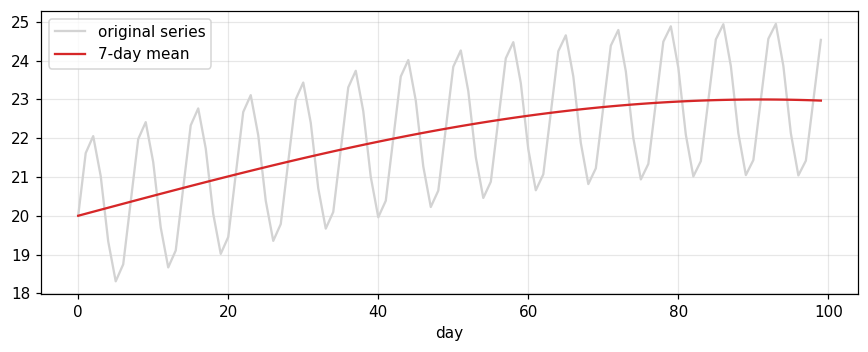
Bracewell mentions that running means smooth meteorological data (p. 33). For a 364-day series with a seasonal trend of amplitude 3 and a weekly cycle of amplitude 2, a 7-day mean (circular) takes the weekly amplitude from 2 to 0 and keeps the seasonal amplitude 2.9982 (theory 2.9982). The two computations, circular convolution and FFT, agree.

Matrix packages and convolution

In computer packages based on matrix operations, convolution is often constructed as the product of a square matrix and a column vector, and the time lost to inefficiency is deemed negligible (p. 38). Current practice uses dedicated functions (convolve, fftconvolve) because they pick a sensible method by length.

Self-check, part 4

• How many terms does the convolution of sequences of lengths 12 and 5 have in full and valid modes?
• Why does multiplying two length-8 FFTs of a length-8 and a length-3 sequence give a wrong result?
• With a very short filter, which method is usually cheaper?

Hints: 16 and 8; because circular convolution wraps the tail; the direct method.

Autocorrelation: definition

The self-convolution of f is \int f(u)f(x-u)du. If prior to multiplication we do not reverse one factor we get the integral below, written f\star f (the five-pointed star, "pentagram"). If f is real then f\star f is an even function, which is not true of convolution in general (pp. 40 to 41).

Normalisation and maximum at the origin

Dividing by the central value gives \gamma(x) with \gamma(0)=1. The appendix proves that the autocorrelation never exceeds its value at the origin: consider \int[f(u)+\varepsilon f(u+x)]^2du\ge0, a quadratic in \varepsilon with no real root, so b^2-4ac<0, the same argument as the Schwarz inequality (pp. 41, 48 to 49). The notebook checks on a random sequence: the largest ratio of a side value to the peak is 0.2821.

Example 1: f=1-x on (0,1)

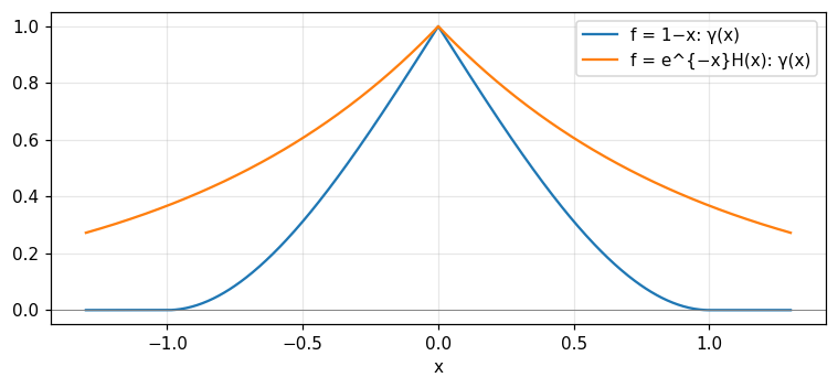
For 0<x<1: \int f(u)f(u+x)du=\tfrac13-\tfrac x2+\tfrac{x^3}6, the central value is \tfrac13, so \gamma(x)=1-\tfrac32|x|+\tfrac12|x|^3 and \gamma=0 for |x|>1. At x=0.25: 0.6328; at x=0.5: 0.3125. The area of the numerator is 0.25, exactly the square of the area of f, (1/2)^2 (pp. 41 to 42).

Example 2: f=e^{-x}H(x)

For f(x)=e^{-x}H(x): \int f(u)f(u+x)du=\tfrac12e^{-|x|} so \gamma(x)=e^{-|x|} (p. 42). At x=1: numerical integration gives 0.3679, exactly e^{-1}. The autocorrelation is even although f lives only on the positive side.

Data that run on: finite segments and the limit C(x)

A function that runs on indefinitely often has no infinite integral. The remedy is to take a segment of length X and replace the values outside it by zero, exactly as in a calculation on a finite quantity of observational data. As X increases \gamma may settle to a limit C(x) (pp. 42 to 43). When the variable is time we write it as the time average \langle V(t)V(t+\tau)\rangle (p. 44).

Three sinusoids: the phases vanish

For V=A\sin(\alpha t+\phi)+B\sin(\beta t+\chi)+C\sin(\gamma t+\psi) the limiting autocorrelation is a superposition of three cosines at the same frequencies with different relative amplitudes and no trace of the phases (pp. 43 to 45). Numbers: A,B,C=2,1,0.5 at 3, 5, 8 Hz; C(0.05) = 0.4093 for two different sets of phases (largest difference 2.2e-16).

Autocorrelation is not reversible

Because the phases are lost, one cannot go back from the autocorrelation to the original function: autocorrelation involves a loss of information. In radio interferometry and X-ray diffraction it is easier to observe the autocorrelation than the function itself, and much ingenuity is spent recovering the lost information (p. 45). Among all functions with the same autocorrelation, the one made of cosines only has a certain uniqueness.

Triple correlation: keeping the arrow of time

Autocorrelation does not know the arrow of time: noise passed through an RC filter e^{-t/RC}H(t) may be statistically different played backwards, yet autocorrelation cannot see it. The triple correlation U(x_1,x_2)=\int f(x)f(x+x_1)f(x+x_2)dx can (pp. 45 to 46). Bracewell notes that \{1,2,3\} and \{3,2,1\} give two different arrays. The notebook confirms: the two sequences have the same autocorrelation (yes) but different triple-correlation arrays (yes); the centre U(0,0)=\sum f^3 = 36 and the sum of all entries (\sum f)^3 = 216.

The array of \{1,2,3\} (rows x_1=-2,\dots,2, columns x_2=-2,\dots,2):

3 6 9 0 0
6 14 22 6 0
9 22 36 14 3
0 6 14 22 6
0 0 3 6 9

Cross correlation and the pentagram

The cross correlation of g and h is g\star h=\int g(u-x)h(u)du: like convolution except that g is only displaced, not reversed. Read it as "g scans h". It is not commutative, but g\star h(x)=h\star g(-x) (p. 46). For complex functions use g^*, and placing the asterisk wrongly yields the conjugate of the standard version (pp. 41, 47).

The notebook checks the relation with discrete sequences: it holds (yes), and g\star h\ne h\star g in general (yes).

The energy spectrum

The squared modulus of the transform, |F(s)|^2, is the energy spectrum. There is no one-to-one relation with f: the phase is needed too. The information lost is of exactly the same character as that lost when autocorrelation stands in for the function, and the autocorrelation theorem (chapter 6) expresses this equivalence (p. 47). The notebook checks the discrete version: the inverse transform of |X|^2 equals the circular autocorrelation (deviation 7.1e-15), and two signals with different phases have the same energy spectrum (deviation 2.3e-10).

The cumulative energy spectrum and spectral lines

Since |F|^2 is energy density per unit s, a spectral line carrying finite energy makes the density infinite. We use the cumulative spectrum \int_0^s|F|^2ds: each line is a finite discontinuity (Fig. 3.12, pp. 47 to 48). Numbers: a signal made of a 50 Hz wave of amplitude 3 plus noise has cumulative energy fraction 0.005 below 49 Hz and 0.951 above 51 Hz: the step at the 50 Hz line is 0.946 of the total energy.

A pulse sequence with good autocorrelation: \{1100101\}

Problem 1(j), (k) and Pettit's paper (1967) in the bibliography point at pulse sequences with good autocorrelation properties. For \{1,1,0,0,1,0,1\} the linear autocorrelation has peak 4 at the origin and largest side value 1; the circular autocorrelation equals 2 at every nonzero shift, almost flat. This property is why such sequences are used in radar and synchronisation.

Takeaways

• Convolution has four pictures (area, smoothing, superposition, folding) and behaves like multiplication: commutative, associative, distributive.
• For unit areas, convolution multiplies areas and adds variances; repeated convolution tends to a Gaussian.
• The serial product is polynomial multiplication; check it by sum and length; invert it by serial division or the table of inverses.
• By machine: the direct code needs l_fl_g multiplications; an FFT must be zero-padded to avoid wrap-around.
• Autocorrelation peaks at the origin, is even for real functions and loses phase; triple correlation keeps the arrow of time; the energy spectrum |F|^2 is equivalent to autocorrelation.

References

R. N. Bracewell, The Fourier Transform and Its Applications, 3rd ed., McGraw-Hill, 2000, chapter 3 (pp. 24 to 50, including the appendix, bibliography and problem 1).
M. Barkat, Signal Detection and Estimation, 2nd ed., Artech House, 2005, sections 3.3 and 3.5, cited only in the cross-reference.
The content was written with AI assistance (Claude) and then checked. Every number is produced by a Jupyter notebook and cross-checked by two independent methods; page citations come from the OCR text of the two source books. Mistakes may remain, so please report them.
R. N. Bracewell, The Fourier Transform and Its Applications, 3rd ed., McGraw-Hill, 2000.
M. Barkat, Signal Detection and Estimation, 2nd ed., Artech House, 2005.
This site only summarises, explains and checks numbers; please read the original books through a library or the publisher.
Contribute
Report errors, suggest modules or translations in the GitHub repository, and fork or clone it for your own study. Please credit the source when sharing.