Notation for useful functions: Π, Λ, H, sgn, sinc, Gaussian

Notation for useful functions: Π, Λ, H, sgn, sinc, Gaussian

• Write piecewise functions with \Pi, \Lambda, H, \text{sgn}, R instead of case-by-case conditions.
• Use the Gaussian normalisation e^{-\pi x^2} and read its dispersion parameters.
• State the properties of \text{sinc} and \text{sinc}^2: zeros, area, cutoff, role as a low-pass filter.
• Understand why convolution with H is integration, and why H(0) rarely needs stating.
• Compare rectangular, triangular and Gaussian windows through the sidelobes of their transforms.

Use the buttons, the dots or the ← → keys to move between slides.

The problem: functions given graphically

The function f(x) equal to 0 for x<0, x for 0\le x\le1 and 1 for x>1 is simple yet awkward to write piecewise, compared with the compact expression 1+x^2. Physically a "sloping step function" may be at least as simple as a smoother function (Bracewell, p. 55).

Fourier and functions given by a graph

Fourier himself was concerned with representing functions given graphically, and according to the English mathematician and historian E. W. Hobson was the first fully to grasp that a single function may consist of detached portions given arbitrarily by a graph (p. 55). This chapter introduces notation to regain compactness and clarity.

The rectangle function \Pi(x)

The rectangle function of unit height and base, centred at the origin (Fig. 4.1, pp. 55 to 56):

Multiplying by \Pi gates a segment

f(x)=\Pi(x)\cos\pi x is compact notation for a function equal to \cos\pi x in |x|<\tfrac12 and 0 outside (Fig. 4.2). Multiplying by \Pi selects ("gates") a segment of any function. The energy of that segment is \int\Pi(x)\cos^2\pi x\,dx = 0.5 (p. 56).

A displaced rectangle of height h and base b

The function h\,\Pi[(x-c)/b] is a rectangle of height h and base b centred at x=c (Fig. 4.3). Purely by multiplying by a suitably displaced rectangle we can select any segment with any amplitude and reduce the rest to zero (p. 56). Example h=3, b=2, c=1: area hb = 6, numerical integration agrees.

Where the rectangle appears: running means and filtering

• Through convolution it gives running means (module 3).
• In the frequency domain multiplying by it is ideal low-pass filtering.
• It is "Dirichlet's discontinuous factor" in the theory of convergence of Fourier series.
• Other names: rect x, gate function, window function, boxcar function (p. 57).

The value at the jump hardly matters

Bracewell almost never states \Pi(\pm\tfrac12), and it is undesirable to emphasise the value \tfrac12 halfway up the jump when drawing, like a high-quality oscillogram that never shows extra brightening halfway up the discontinuity (p. 57). The reason: a single point does not change an integral. Measured: the area with \Pi(\pm\tfrac12)=0, \tfrac12 or 1 differs by at most 2.0e-04, the size of the grid error.

The triangle function \Lambda(x)

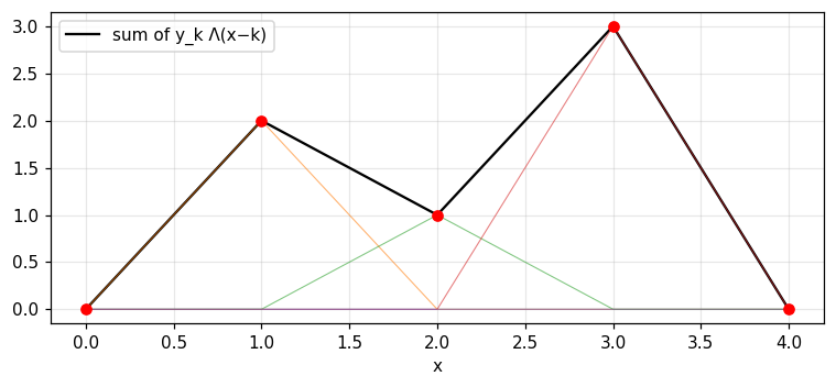
The triangle function has unit height and area. It gains its importance largely from being the self-convolution of \Pi(x), and it gives compact notation for polygonal functions, continuous functions made of linear segments (p. 57). h\Lambda(x/b) has height h, base 2b and area hb.

Numerical test: \Lambda=\Pi*\Pi and polygonal functions

The numerical convolution of \Pi with itself on a fine grid deviates from 1-|x| by at most 1.1e-16, area 1. The polygonal function through (0,0),(1,2),(2,1),(3,3),(4,0) equals \sum y_k\Lambda(x-k): deviation from interp at most 1.1e-16, and at x=2.5 it equals 2.

Four exponentials

Fig. 4.5 shows from left to right: a rising exponential, a falling exponential, a truncated falling exponential and a double-sided falling exponential (p. 57).

Bracewell's Gaussian normalisation

The function \exp(-\pi x^2) is chosen so that both the central ordinate and the area under the curve equal 1, and its Fourier transform is the same normalised Gaussian (p. 58). The notebook measures area 1, central ordinate 1, and the mean of x^2 equal to 0.1592.

The statistical form and the probability ordinate

In statistics the Gaussian is the "normal (error) distribution with zero mean", normalised so the area and standard deviation are 1. For standard deviation \sigma the probability ordinate is \frac{1}{\sigma\sqrt{2\pi}}e^{-x^2/2\sigma^2} with central ordinate 0.3989/\sigma (p. 58). Compared with e^{-\pi x^2} we have \sigma=(2\pi)^{-1/2} = 0.3989.

The error integral erf, erfc and the probability integral

The error integral \text{erf}\,x=\frac{2}{\sqrt\pi}\int_0^xe^{-t^2}dt with complement \text{erfc}\,x=1-\text{erf}\,x; the probability integral a(x) is widely tabulated. For the book's Gaussian, \int_0^xe^{-\pi t^2}dt=\tfrac12\text{erf}(\sqrt\pi\,x) (pp. 58 to 59). At x=1: numerical integration and the formula give 0.4939.

Dispersion parameters of e^{-\pi x^2}

The book lists five parameters (p. 59); the notebook recomputes each by two methods (closed form and numerical integration or root finding):

What percentage lies within each parameter?

The probable error characterises the middle 50 percent of a set of measurements: "the students have an average height of 165 ± 10 cm" means half of the students are in 155 to 175 cm unless another measure of spread is specified (p. 59). For a normal distribution the percentage within one standard deviation is 68.27, within the mean absolute error 57.51, within the semi-width to half-peak 76.1, within the semi-equivalent width 78.99.

Two dimensions and the Rayleigh distribution

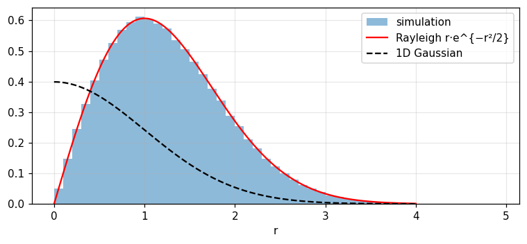
The two-dimensional Gaussian e^{-\pi(x^2+y^2)} is still self-transforming, with unit central ordinate and unit volume. With circular symmetry the probability of finding the radial distance between r and r+dr is 2\pi r\,dr times the ordinate, so R(r)=\frac{r}{\sigma^2}e^{-r^2/2\sigma^2}. This is Rayleigh's distribution (pp. 59 to 60).

The drunkard's walk: the paradox of the peak away from the origin

Rayleigh's drunkard's-walk problem: each step is in an arbitrary direction. After a long time the probability at (x,y) is a two-dimensional Gaussian (peak at the origin) yet the probability at distance r is Rayleigh (peak away from the origin). The two sound contradictory and Bracewell invites you to contemplate it (p. 60). A simulation of 400 000 points: mean distance 1.253 (theory 1.2533), peak at 0.98, and 0.395 of the points lie within r<\sigma (theory 0.3935).

Gaussian sequences for transforms in the limit

The sequence \exp(-\pi\tau^2x^2) as \tau\to0 multiplies functions whose integrals do not converge; the limit is 1. The sequence |\tau|^{-1}\exp(-\pi x^2/\tau^2) recovers ordinary functions, in cases of impulsive behaviour, by convolution. The Gaussian suits this because all its derivatives are continuous and it dies away faster than any power of x (p. 60). Measured: \int\cos x\,|\tau|^{-1}e^{-\pi x^2/\tau^2}dx=e^{-\tau^2/4\pi} equals 0.9235 (\tau=1), 0.9803 (\tau=0.5), 0.9992 (\tau=0.1), tending to \cos0=1.

The unit step H(x)

H(x) is 0 for x<0, 1 for x>0 (and usually \tfrac12 at 0). It represents voltages suddenly switched on or forces that begin to act at a definite time and are constant thereafter (Fig. 4.8, p. 61). Multiplying a function by H reduces it to zero on the negative side and leaves it intact on the positive side.

Switching notation

A sinusoid switched on at t=0 is \sin t\,H(t) (Fig. 4.10). A voltage zero until t_0 and then jumping to a steady E is EH(t-t_0) (Fig. 4.11). Any function with a jump decomposes into a continuous function plus a suitably displaced step (pp. 61 to 62).

\Pi is made of steps alone

The rectangle has two unit discontinuities, one positive and one negative; remove them and nothing remains. Hence \Pi(x)=H(x+\tfrac12)-H(x-\tfrac12) (Fig. 4.9, p. 61). The notebook checks it numerically on a grid: yes, even at x=\pm\tfrac12 with H(0)=\tfrac12.

The ramp R(x)=xH(x)

(F/m)R(t) is the velocity of a mass m to which a steady force FH(t) has been applied, or the current in a coil of inductance m across which the potential difference is FH(t). R is the integral of H and H is the derivative of R (Fig. 4.12, pp. 61 to 62). Notebook: the numerical convolution H*H at x=2 gives 2, exactly R(2).

Convolution with H is integration

Because H(x-x') is zero for x'>x, integrals with variable limits become constant-limit integrals: \int_{-\infty}^xf(x')dx'=\int f(x')H(x-x')dx'. Hence H*f is the integral of f (Fig. 4.13, pp. 62 to 63). With f=e^{-\pi x^2} at x=0.5: numerical convolution with a step gives 0.8945, exactly \tfrac12[1+\text{erf}(\sqrt\pi\,x)] (largest deviation 0.001).

The value H(0) and consistency

It is usually unimportant to define H(0), but for compatibility with the theory of single-valued functions it is desirable to assign \tfrac12. Then R'(0+)=1, R'(0-)=0 and the symmetric derivative at 0 equals \tfrac12; the Fourier integral, when it converges at a point of discontinuity, also gives the midvalue (p. 63). Measured: [R(\Delta)-R(-\Delta)]/2\Delta = 0.5.

Choosing H(0)=0 and null functions

There is no obligation to take H(0)=\tfrac12; it is sometimes taken as zero, a natural consequence of the view \hat H(x)=\lim_{\tau\to0}(1-e^{-x/\tau})H(x) (Fig. 4.14). Then H=\hat H+\tfrac12\delta^{\circ} with \delta^{\circ} a null function: zero everywhere except the origin, with integral always zero (pp. 63 to 64). Measured: \int(H-\hat H)\,dx=\tau = 0.01 for \tau=0.01, tending to 0.

Continuous approximations to H

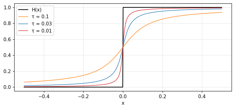
The book lists many smooth approximations tending to H(x) as \tau\to0, for example \tfrac12+\frac1\pi\arctan\frac x\tau, the integral of a Lorentzian (p. 64). At x=0.1: with \tau=0.1 we get 0.75, with \tau=0.01 we get 0.9683, approaching 1. The difference between H and any version with H(0)\ne\tfrac12 is a null function, invisible to physical measurements of finite resolving power, so it is more graceful not to mention H(0) (pp. 64 to 65).

The sign function \text{sgn}\,x

\text{sgn}\,x equals +1 or -1 according to the sign of x, and \text{sgn}\,x=2H(x)-1 (a jump of 2). Unlike H it is an odd function, whereas H has both an even part (\tfrac12) and an odd part (\tfrac12\text{sgn}\,x): the notebook confirms yes. Moreover \lim\int_{-a}^{a}\text{sgn}\,x\,dx=0 while \int_{-a}^{a}H\,dx=a does not exist as a\to\infty (p. 65).

Definition and properties of \text{sinc}\,x

\text{sinc}\,x=\sin\pi x/\pi x has \text{sinc}\,0=1, vanishes at every nonzero integer, and has total area 1. The word "sinc" appears in Woodward (1953) and has achieved some currency; a table is on p. 508 (pp. 65 to 66). Notebook: \text{sinc}(3) = 0; \int_0^{100}\text{sinc} = 0.499, tending to \tfrac12 (half of area 1).

Sinc and \Pi are a transform pair

The unique properties of sinc go back to its spectral character: it contains components of all frequencies up to a limit and none beyond, with a flat spectrum up to the cutoff. By the choice of notation, \text{sinc}\,x and \Pi(s) are a Fourier transform pair, so the cutoff of sinc is 0.5 cycles per unit of x (p. 66). Measured: \int_{-1/2}^{1/2}e^{i2\pi sx}ds at x=0.3 is 0.8584, exactly \text{sinc}(0.3).

Sinc in convolution: ideal low-pass filtering and interpolation

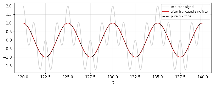
When sinc enters convolution it performs ideal low-pass filtering: it removes all components above its cutoff and leaves all below unaltered, and under special circumstances (the sampling theorem, chapter 10) it performs interpolation (p. 66). Test: the signal \cos2\pi(0.2)t+\cos2\pi(0.8)t convolved with a truncated sinc: the gain at 0.2 is 0.998 and at 0.8 is 0.001; a brick-wall filter through the FFT gives 1 and 0.001.

The integral of sinc: the sine integral \text{Si}

With \text{Si}\,x=\int_0^x\frac{\sin u}{u}du we have \int_0^x\text{sinc}\,u\,du=\text{Si}(\pi x)/\pi, \text{sinc}\,x=\frac{d}{dx}\frac{\text{Si}(\pi x)}{\pi} and H*\text{sinc}=\tfrac12+\text{Si}(\pi x)/\pi (Fig. 4.16, pp. 66 to 67). The integral curve overshoots 1 before returning: the maximum is 1.0895 at x=1, a Gibbs-type overshoot.

Sinc squared

\text{sinc}^2x represents the power radiation pattern of a uniformly excited antenna, or the intensity of light in the Fraunhofer diffraction pattern of a slit. It has a cutoff spectrum since squaring cannot generate frequencies higher than the sum-frequency of any pair of constituents. Its transform is \Lambda(s), with cutoff one cycle per unit (Fig. 4.17, pp. 66 to 68). Measured: \text{sinc}^2(0.5) = 0.4053 by both \int\Lambda(s)e^{i2\pi s/2}ds and the formula; area 1.

The two-dimensional analogue: \text{jinc}

In two dimensions the analogous function is J_1(\pi r)/2r, which has unit volume, a central value \pi/4 and a two-dimensional transform equal to a circular pulse. Another generalisation with analogous filtering and interpolating properties is \text{sinc}\,x\,\text{sinc}\,y, with transform \Pi(u)\Pi(v) (p. 68). Measured: the central value 0.7854 and the first zero at r = 1.2197, the radius of the Airy disc in optics.

Graphical conventions

For clarity, theorems on Fourier transforms are illustrated by real examples where possible, marking the points where the abscissa and ordinate equal unity. Purely imaginary quantities are always drawn dashed, so complex quantities are shown unambiguously by real and imaginary parts (Fig. 4.18); one may also plot modulus and phase (Fig. 4.19), draw in three dimensions (Fig. 4.20) or plot the values of F(s) on the complex plane (Fig. 4.21) (pp. 68 to 69).

Table 4.1: special symbols

Bracewell collects the symbols (p. 70):

Rewriting the opening function

The function f(x) from the start of the chapter (0, then x on [0,1], then 1) equals R(x)-R(x-1), and also x\,\Pi(x-\tfrac12)+H(x-1). All three writings coincide on a grid (yes); at x=0.4 it equals 0.4.

Transform pairs for the functions just learned

The book tabulates these pairs in chapter 22; here we check them numerically at s=0.3 (numerical integral versus formula; 5 of 5 pairs hold):

Three windows: rectangle, triangle, Gaussian

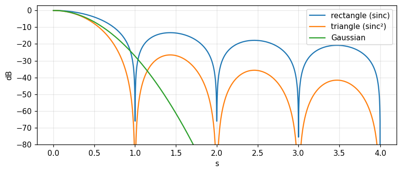
Cutting a signal with a window multiplies the spectrum by the window's transform's convolution. The transform of \Pi is \text{sinc}\,s, of \Lambda is \text{sinc}^2s, of a Gaussian a Gaussian. The first sidelobe of \text{sinc} has magnitude 0.2172 (-13.26 dB), that of \text{sinc}^2 only 0.0472 (-26.52 dB), and the Gaussian has none. That is why leakage in module 1 is heavy with the rectangular window.

The trade-off: sidelobes versus main-lobe width

The triangular window lowers the sidelobes but widens the main lobe (a null at |s|=1 versus 0.5 for the rectangle at the same base b=1; a triangle of base 2 has its null at 1). No window has both low sidelobes and a narrow main lobe; this is a manifestation of the uncertainty relation (chapter 8).

A scanning slit is convolution with \Pi

The optical sound track on old motion-picture film is scanned by a slit of width w, and the scanning introduces convolution with a rectangle of width w (chapter 3 problem 23, p. 53). For a sinusoidal track of period p=1: a slit w=0.25 keeps 0.9003, w=0.5 keeps 0.6366, w=1 keeps 0 (the tone is wiped out completely). The gain is \text{sinc}(wf_0).

An L-point running mean and sinc

A running mean is convolution with \Pi, so its frequency response is sinc, more precisely the Dirichlet kernel for a discrete sequence. For L=8 at f=0.05 cycles per sample: the exact value is 0.7599 (measured with freqz and by the formula) and the sinc approximation 0.7568. The approximation is good for large L and small f.

Tips for using the notation

• Set H(0)=\tfrac12 or do not mention it; do not emphasise the value at a jump when drawing (pp. 57, 63).
• Use H to turn variable integration limits into constant ones (p. 62).
• Choose e^{-\pi x^2} when self-transformation is wanted; convert to the statistical form with \sigma=(2\pi)^{-1/2} (p. 58).
• Draw imaginary quantities dashed (p. 68).

Cross-reference to Barkat

The Gaussian and Rayleigh of this module are the distributions of Barkat sections 2.3.2 (Normal) and 2.3.6 (Rayleigh, Rice, Maxwell). Barkat uses the step and the impulse in section 1.3.1 to write the cumulative distribution and density of a discrete random variable: F_X(x)=\sum_kP_k\,H(x-x_k). Module 11 uses both.

Self-check

• Write \Lambda(x) using \Pi and \Pi(x) using H.
• Where does sinc vanish and what is its cutoff?
• Why does the Rayleigh peak lie away from the origin although the 2D Gaussian peaks there?

Hints: \Pi*\Pi and H(x+\tfrac12)-H(x-\tfrac12); nonzero integers and 0.5; because the ring area 2\pi r\,dr grows with r.

Takeaways

• \Pi is a gate, \Lambda=\Pi*\Pi is the triangle, and combinations of H and R build every polygonal and switching function.
• The Gaussian e^{-\pi x^2} has central ordinate and area 1 and is self-transforming; \sigma=(2\pi)^{-1/2}.
• Convolution with H is integration; H(0) hardly needs stating; \text{sgn}\,x=2H-1 is odd.
• \text{sinc}\,x\supset\Pi(s): zeros at integers, cutoff 0.5, ideal low-pass; \text{sinc}^2\supset\Lambda with cutoff 1.
• The triangular window lowers sidelobes compared with the rectangle, at the cost of a wider main lobe.

References

R. N. Bracewell, The Fourier Transform and Its Applications, 3rd ed., McGraw-Hill, 2000, chapter 4 (pp. 55 to 70) and chapter 3, problem 23 (p. 53).
M. Barkat, Signal Detection and Estimation, 2nd ed., Artech House, 2005, sections 1.3.1, 2.3.2 and 2.3.6, cited only in the cross-reference.
The content was written with AI assistance (Claude) and then checked. Every number is produced by a Jupyter notebook and cross-checked by two independent methods; page citations come from the OCR text of the two source books. Mistakes may remain, so please report them.
R. N. Bracewell, The Fourier Transform and Its Applications, 3rd ed., McGraw-Hill, 2000.
M. Barkat, Signal Detection and Estimation, 2nd ed., Artech House, 2005.
This site only summarises, explains and checks numbers; please read the original books through a library or the publisher.
Contribute
Report errors, suggest modules or translations in the GitHub repository, and fork or clone it for your own study. Please credit the source when sharing.