The impulse symbol: \delta, sifting, shah and generalized functions

The impulse symbol: \delta, sifting, shah and generalized functions

• Explain \delta(x) as the limit of unit-area pulses and why the pulse shape does not matter.
• Use the sifting property, the scaling \delta(ax), and take care with x\delta(x).
• Use \text{III}(x) for sampling and replication, and the even and odd pairs for finite differences.
• Compute with \delta', \delta'', null functions and multidimensional impulses.
• Understand a generalized function as a class of regular sequences, with derivatives defined by integration by parts.

Use the buttons, the dots or the ← → keys to move between slides.

The impulse: only the integral matters

We need notation for intense unit-area pulses so brief that measuring equipment of a given resolving power cannot tell them from even briefer ones. Mechanics calls this an "impulse". The important attribute is its integral; the precise details of its form are unimportant (Bracewell, p. 74).

History of the symbol \delta(x)

The idea has been current for a century or more in mathematical circles: van der Pol and Bremmer (1955) cite examples from Hermite, Cauchy, Poisson, Kirchhoff, Helmholtz, Kelvin and Heaviside. The notation \delta(x) was first used by G. Kirchhoff and introduced into quantum mechanics by Dirac in 1927 (p. 74).

Things that do not exist but are useful

Point masses, point charges, point sources, concentrated forces, line sources and surface charges are familiar and accepted entities in physics, though they do not exist. Their conceptual value stems from the fact that the impulse response, the effect associated with the impulse, may be indistinguishable, given measuring equipment of specified resolving power, from the response due to a physically realisable pulse (p. 74).

Definition: not a function

We wish to write \delta(x)=0 for x\ne0 and \int\delta=1, but the impulse symbol does not represent a function in the sense of analysis. Dirac called it an "improper function", and the integral above has no meaning until a convention of interpretation is declared. Here it means the limit of \int\tau^{-1}\Pi(x/\tau)dx as \tau\to0 (pp. 74 to 75).

• \tau^{-1}\Pi(x/\tau)rectangle of height \tau^{-1}, base \tau, unit area

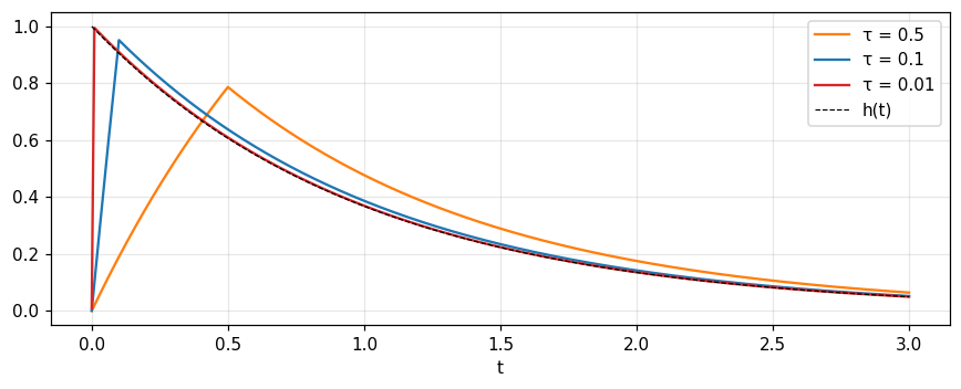
An RC low-pass circuit: the pulse shape gradually stops mattering

Feed voltage pulses into a low-pass filter: the transient response settles to a definite form as the pulses shorten, independent of the input pulse shape, because the high-frequency components that distinguish the pulses produce negligible response (p. 75). For an RC circuit with h(t)=e^{-t}H(t) and three unit-area pulses (rectangle, triangle, two small pulses) of width \tau: at t=1 the spread among the three responses is 0.009 for \tau=0.5, 0.0003 for \tau=0.1 and 0 for \tau=0.01.

The relation between \delta and the step

Since \int_{-\infty}^x\delta(x')dx' is 1 for x>0 and 0 for x<0, we have \int_{-\infty}^x\delta=H(x). To interpret it, replace \delta by the sequence \tau^{-1}\Pi(x/\tau): the integrals are ramp-step functions (Fig. 5.1); fix x and let \tau\to0 (pp. 75 to 77). At x=0.1: \tau=0.5 gives 0.7, \tau=0.1 gives 1; at x=-0.1: 0.3 and 0.

What "the derivative of the step is the impulse" means

The step has no derivative at the origin, so the statement is shorthand for: the derivatives of a sequence of differentiable functions approaching H(x) constitute a suitable defining sequence for \delta(x). The ramp-step functions of Fig. 5.1 are differentiable and approach H; since the step is always 1 the area under each derivative is 1, qualifying it as a unit-impulse sequence (p. 77).

Many different sequences define the same \delta

Bracewell lists sequences as \tau approaches zero through positive values (pp. 77 to 78): a displaced rectangle (left edge at the origin, common in switched circuits), the Gaussian (derivatives of all orders exist), the triangle (continuous, zero outside |x|<\tau), \tau^{-1}\text{sinc}(x/\tau) (does not die out yet serves), the resonance profile \tau/[\pi(x^2+\tau^2)] (decays slowly), and a smooth compactly supported bump. The table gives \int f\,\delta_\tau\,dx with f=\cos x+\tfrac12\sin2x (so f(0)=1):

All symmetric shapes tend to 1; the left-edge shape tends to f(0+) at a discontinuity so it differs a little until \tau is small.

Self-check, part 1

• Why can an RC circuit not tell very brief input pulses of different shapes apart?
• Why is "the derivative of the step is the impulse" only shorthand?
• Which sequence in the table above differs from 1 while \tau is not small, and why?

Hints: because high-frequency components produce almost no response; because the step has no derivative at the origin; the left-edge rectangle, because it sifts f from just to the right.

The sifting property

Replace \delta by \tau^{-1}\Pi(x/\tau), multiply by f, integrate and let \tau\to0: the area is about \tau^{-1} times the shaded part, whose average height is near f(0) and width \tau, so it tends to f(0). The operation "sifts" out a single value of f. The pulse shape does not matter, only its integral counts (p. 79).

Convolution with \delta changes nothing

Written as a convolution, \delta(x)*f(x)=f(x)*\delta(x)=f(x). If f has a jump at x=0 the sifting integral has limiting value \tfrac12[f(0+)+f(0-)], so more generally \delta*f=\tfrac12[f(x+)+f(x-)]; it differs from f only by a null function (p. 80). Measured with f=e^{-x}H(x): the centred sequence gives 0.5, the left-edge sequence gives 1 at the jump.

The left-edge sequence sifts f(x+)

The asymmetric rectangular sequence \tau^{-1}\Pi[(x-\tau/2)/\tau] sifts out f(x+). At points of discontinuity this sequence gives a different result. In transient analysis, where discontinuities at the switching instant t=0 are particularly common, the choice of sequence can appear to give different answers, but the difference can only be instantaneous (p. 80).

Scaling: \delta(ax)=|a|^{-1}\delta(x)

Compressing the scale of x by a reduces the area of pulses that previously had unit area, so the strength of the impulse is reduced by |a|. The modulus allows for \delta(-x)=\delta(x) (p. 80). Measured: \int f\,\tau^{-1}\Pi(3x/\tau)dx with \tau=0.01 equals 0.3333, close to f(0)/3.

Multiplying by a continuous function: f(x)\delta(x)=f(0)\delta(x)

If f is continuous at 0 then f(x)\delta(x)=f(0)\delta(x) (p. 81). Numerical check with the test function g=e^{-x^2} and a Gaussian sequence \tau=0.01: \int f\delta_\tau g\,dx = 1, exactly f(0)g(0)=1.

x\delta(x)=0: true, but qualified

From sifting with f=x, \int x\delta(x)dx=0, and one writes x\delta(x)=0. But contemplating the prelimit graphs, this equation conceals a nonvanishing component reminiscent of the Gibbs phenomenon: \lim_{\tau\to0}[x\tau^{-1}\Pi(x/\tau)]=0 for all x, yet its maximum is always \tfrac12 and its minimum -\tfrac12 (p. 81). Measured: maximum 0.5 for both \tau=0.1 and \tau=0.001.

The shah impulse train \text{III}(x)

An infinite sequence of unit impulses spaced by 1 (Fig. 5.4). Every reservation about \delta applies, and more: infinitely many infinite discontinuities and a nonconvergent infinite integral, so all conditions for a Fourier transform are violated; yet it is extremely useful and easy to manipulate (pp. 81 to 82). Obvious properties: period 1, even, \text{III}(x-\tfrac12)=\text{III}(x+\tfrac12).

Sampling: multiplying by shah

Multiplying f(x) by \text{III}(x) samples it at unit intervals: \text{III}(x)f(x)=\sum f(n)\delta(x-n). The information between the integers is lost but the values at integers are preserved. Shah serves antenna-array patterns, diffraction gratings, raster scanning in television and radar, pulse modulation, data sampling, Fourier series and tabular computing (p. 82). The sum of samples \sum_nf(n) for f=e^{-\pi x^2} is 1.0864.

Replication: convolving with shah

\text{III}*f=\sum f(x-n): f appears in replica at unit intervals on both sides; if f is more than one unit wide the replicas overlap (Fig. 5.6). This twofold character is no accident: \text{III} is its own Fourier transform (in the limit), making it twice as useful (pp. 82 to 83). For f=e^{-\pi x^2}, (\text{III}*f)(0.5) = 0.9136, computed both by the direct sum and by the Fourier series \sum(-1)^ke^{-\pi k^2}.

The \text{III}(ax) trap: impulse strength

Squeezing shah by 2 into \text{III}(2x) packs the impulses twice as closely, but for algebraic consistency their strength drops by the same factor: \text{III}(ax)=|a|^{-1}\sum\delta(x-n/a). If it is stretched so that the spacing is X then \text{III}(x/X) does not have unit strength: unit impulses spaced X are X^{-1}\text{III}(x/X) (p. 83). Measured with f=e^{-\pi x^2} (area 1): \sum f(nX) = 1.0864 (X=1) and 2 (X=0.5, twice too large because the factor X is missing), while X\sum f(nX) = 1 (X=0.5), the area.

Poisson duality: shah is self-transforming

Since \text{III}\supset\text{III}, the sum of samples of f equals the sum of samples of F: \sum f(n)=\sum F(k). With f=e^{-\pi x^2/4} having F=2e^{-4\pi s^2}: the left side is 2.000014 and the right side 2.000014, equal to rounding error. This is the Poisson summation formula chapter 10 will use for the sampling theorem.

Self-check, part 2

• Why does x\delta(x)=0 still leave a maximum of \tfrac12 before the limit?
• How are unit impulses spaced X represented?
• Why does \text{III} both sample and replicate?

Hints: because x\tau^{-1}\Pi(x/\tau) reaches \tfrac12 at the edge; X^{-1}\text{III}(x/X); because it is self-transforming.

The even and odd impulse pairs

Bracewell defines (Fig. 5.7, special symbols in Table 4.1; written here as \mu and \nu):

They matter because of their transform relation to cosine and sine: \mu(x)\supset\cos\pi s, \cos\pi x\supset\mu(s), and \nu(x)\supset i\sin\pi s, \sin\pi x\supset i\nu(s) (p. 84). Notebook: the numerical transform of \mu at s=0.3 is 0.5878, exactly \cos0.3\pi.

The even pair duplicates a function

Convolving with \mu gives \mu*f=\tfrac12f(x+\tfrac12)+\tfrac12f(x-\tfrac12), the mean of two displaced copies (Fig. 5.8). Normalising to unit area has advantages; occasionally two unit impulses would be preferable (p. 84). With f=e^{-\pi x^2} at x=0: 0.4559.

Finite difference through the odd pair

Defining the finite difference \Delta f(x)=f(x+\tfrac12)-f(x-\tfrac12) we have \Delta f=2\nu*f, i.e. the operator \Delta=2\nu* (pp. 84 to 85). Numerical check: for f=\sin x, \Delta f(0)=2\sin\tfrac12 = 0.9589; for f=e^{-\pi x^2} the transform of \Delta f is 2i\sin(\pi s)F(s), of magnitude 1.2195 at s=0.3 by both numerical integration and the formula.

The first derivative \delta'(x): the dipole

\delta'(x)=\frac{d}{dx}\delta(x) evokes an infinitesimal dipole in electrostatics, a familiar and easy picture. The notation \delta' carries that facility into mathematics, but we cannot ask a function to go positively infinite just left of the origin, negatively infinite just right, and zero everywhere else. We would also wish to write \delta'(0)=0 (p. 85).

Rigorous reading: derivatives of a pulse sequence

We fall back on pulse sequences as for \delta and consider their derivatives (Fig. 5.9). For example \int\delta'(x)dx=0 is shorthand for \lim\int[\text{derivative of the pulse}]dx=0. The exact pulse form is unimportant, even a rectangle will do, but in later work a smooth pulse may offer an advantage (pp. 85 to 86). Derivative sifting: \int\delta'(x)f(x)dx=-f'(0); with the Gaussian sequence \tau=0.05 and f=\cos x+\tfrac12\sin2x it gives -0.9992, equal to -\int\delta_\tau f' (difference 4.2e-15).

Properties of \delta'

The accompanying properties (p. 86): \int x\delta'(x)dx=-1, \int|\delta'(x)|dx=\infty, \delta'(-x)=-\delta'(x), x\delta'(x)=-\delta(x), and f(x)\delta'(x)=f(0)\delta'(x)-f'(0)\delta(x). Measured: \int x\delta'_\tau dx = -1; \int|\delta'_\tau|dx = 20 for \tau=0.1 and 200 for \tau=0.01, growing like 2/\tau: no finite limit.

Higher derivatives

For higher-order derivatives (p. 87): \int\delta''(x)dx=0, \int x^2\delta''(x)dx=2, x^n\delta^{(n)}(x)=(-1)^nn!\,\delta(x), and \int\delta^{(n)}(x)f(x)dx=(-1)^nf^{(n)}(0). Measured: \int x^2\delta''_\tau dx = 2; with f=\cos x+\tfrac12\sin2x, \int\delta''f = -1, exactly f''(0)=-1.

Null functions

Null functions are known chiefly for having Fourier transforms that are zero while not themselves identically zero. By definition f is null if \int_a^bf\,dx=0 for all a,b. Lerch's theorem: if two functions have the same transform then their difference is a null function. An example is \delta^{\circ}(x), 0 for x\ne0 and 1 at x=0; it describes the current taken by a series combination of a resistance and a capacitance from a battery, as the capacitance approaches zero (p. 87). Measured: the area of a single point of height 1 on a grid of step 10^{-3} and 10^{-6} is 1e-03 and 1e-06, tending to 0.

Self-check, part 3

• Compute \int\delta'(x)\cos x\,dx and \int\delta''(x)\cos x\,dx.
• Why is \int|\delta'|=\infty although \int\delta'=0?
• What is the Fourier transform of a null function?

Hints: 0 and -1; because the positive and negative halves each grow like 1/\tau; zero.

Two- and three-dimensional impulses

^2\delta(x,y) describes the pressure distribution over the plane when a concentrated unit force is applied at the origin; ^3\delta(x,y,z) describes the charge density in a volume containing a unit charge at (0,0,0). Properties are established with sequences such as \tau^{-2}\Pi(x/\tau)\Pi(y/\tau) of unit volume (p. 89).

Radial and cylindrical forms

With r^2=x^2+y^2, ^2\delta(x,y)=\delta(r)/\pi r. In three dimensions, ^3\delta(x,y,z)=\delta(x)\delta(y)\delta(z)={}^2\delta(x,y)\delta(z), with matching forms in cylindrical and spherical coordinates (pp. 89 to 90). Measured: the integral over the plane (2\pi r\,dr) of a two-dimensional Gaussian sequence (\tau=0.1) equals 1.

The bed of nails ^2\text{III}(x,y)

For two-dimensional arrays use the bed-of-nails symbol (Fig. 5.12). It factorises: ^2\text{III}(x,y)=\text{III}(x)\text{III}(y), is doubly periodic, and f(x,y)\,{}^2\text{III}=\sum\sum f(m,n)\,{}^2\delta(x-m,y-n): two-dimensionally sampled data and the coefficients of double Fourier series (pp. 90 to 91). Convolving with it gives two-dimensional replicas, as in an array of identical antennas. Measured: \sum\sum e^{-\pi(m^2+n^2)} = 1.1803, the square of the one-dimensional sum 1.0864.

The row of spikes and the grating

Two other important two-dimensional distributions need no new symbols: the row of spikes \text{III}(x)\delta(y) and the grating \text{III}(x) (Fig. 5.14). They form a two-dimensional Fourier transform pair, suitable for discussing the diffraction of light by a row of pinholes or by a diffraction grating (p. 91).

Derivatives of impulses: dipoles and quadrupoles

Interpreted with derivatives of impulses, many forms are familiar electric-charge distributions. \delta'(x) on the (x,y)-plane is a line distribution of dipole moment on the y-axis; in three dimensions a sheet of dipole moment on the (y,z)-plane. A simple dipole at the origin with unit moment along x is -\delta'(x)\delta(y)\delta(z). A simple unit quadrupole is \delta''(x)\delta(y)\delta(z) (pp. 91 to 92).

Use in physical equations

\delta'(x)\delta'(y) represents an electromagnetic radiator with a quatrefoil (clover-leaf) radiation pattern in the (x,y)-plane. All these symbolic expressions may confidently be inserted into Maxwell's equations, the wave equation, Poisson's equation and other fundamental differential equations (p. 92).

Self-check, part 4

• Write ^2\delta(2x,3y) in terms of ^2\delta(x,y).
• How is ^2\text{III}(x,y) related to \text{III}(x) and \text{III}(y)?
• Which impulse represents a unit dipole along x?

Hints: \tfrac16\,{}^2\delta(x,y); the product; -\delta'(x)\delta(y)\delta(z).

Why we need generalized functions

The impulse symbol and combinations such as \text{III} and \mu bring much convenience, one use being to provide derivatives for functions with simple discontinuities. Ordinarily we would say the derivative does not exist; the impulse symbol permits such discontinuities to be accommodated (Bracewell, p. 92). The word "symbol" reminds us these are not functions.

Pure alternating current: the infinitely remote past is convenient

Pure alternating current means an eternal harmonic variation, which cannot be generated. But the response to a variation that is harmonic over an interval and zero outside can be made independent of the switching time to a given precision by waiting long enough. Since the details of switching are irrelevant they may be relegated to the infinitely remote past (pp. 92 to 93). Likewise impulses cannot be generated, but responses to sufficiently brief pulses can be made indistinguishable at finite resolution.

Finite resolution is the key

Precision of measurement is limited by the temporal and spectral resolution of the instrument. That feature is the key to the mathematical interpretation: integrals containing \delta are limits of a sequence of integrals in which \delta is replaced by unit-area rectangular pulses. The limit may exist even though the rectangular pulses grow without limit. The physical situation is a sequence of ever more compact stimuli producing responses that become indistinguishable however high the precision (p. 93).

History of the approach

A satisfactory mathematical formulation was evolved along these lines and is expounded in the books of Lighthill (1958) and Friedman (1956). Lighthill credits Temple with simplifying the presentation; Temple (1953) credits the Polish mathematician Mikusiński (1948) with introducing the presentation in terms of sequences. Schwartz's two volumes (1950, 1951) on the theory of distributions unify partial and special techniques. The idea of sequences was current in physical circles before 1948, going back to G. S. Kirchhoff in 1882 (p. 93).

The class S: particularly well-behaved functions

The class S consists of functions with derivatives of all orders at all points which, with all their derivatives, die off at least as rapidly as |x|^{-N} as |x|\to\infty, however large N. The derivative and the Fourier transform of a function in S are also in S (p. 94). The decay of the transform reflects smoothness: the transform of a Gaussian at s=3 is 5.3e-13, while for the rectangle |\text{sinc}(3.5)| = 0.0909, decaying only like 1/s.

Regular sequences

Among sequences of particularly well-behaved functions we distinguish sequences p_\tau(x) which lead to limits when multiplied by any well-behaved F(x) and integrated: regular sequences. The sequence \tau^{-1}\exp(-\pi x^2/\tau^2) is regular; Fig. 5.15 shows a non-regular example. Unit area is not essential; for instance (1+\tau^{-1})\exp(-x^2/\tau^2) is also regular (pp. 94 to 95).

A generalized function is a class of sequences

A generalized function p(x) is defined by a regular sequence. Since the limit can be the same for more than one sequence, it is finally the class of all equivalent regular sequences. The symbol p(x) stands for an entity different from an ordinary function: it stands for a class of functions and is itself not a function, so when written where ordinary functions are customary the meaning must be stated (p. 95). The sequences \tau^{-1}\Pi(x/\tau) and \tau^{-1}\Lambda(x/\tau) do not strictly define one since they lack derivatives of all orders, but they are usable where only low-order derivatives are needed (pp. 95 to 96).

Proof that \tau^{-1}e^{-\pi x^2/\tau^2}\to\delta

The sequence e^{-\pi\tau^2x^2} defines the generalized function I(x)=1 since \lim\int e^{-\pi\tau^2x^2}F\,dx=\int F\,dx. The sequence \tau^{-1}e^{-\pi x^2/\tau^2} defines \delta: \bigl|\int\tau^{-1}e^{-\pi x^2/\tau^2}[F(x)-F(0)]dx\bigr|\le\max|F'|\int|x|\tau^{-1}e^{-\pi x^2/\tau^2}dx=\tau\max|F'|/\pi, which tends to 0 (p. 96). Measured with F=\cos x, \tau=0.1: the actual deviation 8.0e-04 is below the bound 3.2e-02.

Algebra: adding and differentiating generalized functions

The sum of two regular sequences is regular and independent of the choice of sequences, so p+q is meaningful (pp. 96 to 97). Derivatives are defined through integration by parts: \int p'F\,dx=-\int pF'\,dx, and in general \int p^{(n)}F\,dx=(-1)^n\int pF^{(n)}dx. Since well-behaved F has derivatives of every order, a generalized function has derivatives of every order (pp. 97 to 98).

Differentiating ordinary functions: H'=\delta

An ordinary function of slow growth can also be regarded as a generalized function, so H(x) has a derivative: \int H'F\,dx=-\int H F'\,dx=-\int_0^\infty F'dx=F(0), while \int\delta F\,dx=F(0), hence H'=\delta (p. 98). Measured with F=e^{-x^2}: -\int_0^\infty F' = 1; with the derivative sequence of \tfrac12+\arctan(x/\tau)/\pi (a Lorentzian), \tau=0.1 gives 0.8965 and \tau=0.01 gives 0.9888: converging to 1 but slowly because of the Lorentzian tails.

Cross-reference to Barkat

Barkat, section 1.3.1 (Step and Impulse Functions), uses exactly these tools for random variables: the cumulative distribution of a discrete variable is a sum of steps \sum P_kH(x-x_k) and its density a sum of impulses \sum P_k\delta(x-x_k); mixed variables have both a continuous part and an impulsive part (section 1.3.4). Module 10 merges the two books here.

Self-check, part 5

• How does a generalized function differ from an ordinary function?
• How is the derivative of a generalized function defined?
• Why is H'=\delta although H has no derivative at 0?

Hints: it is a class of regular sequences; by integration by parts; because the derivative is defined through the test -\int HF'=F(0).

Takeaways

• \delta is shorthand for a sequence of unit-area pulses; the pulse shape does not matter, only the integral.
• Sifting: \int\delta f=f(0); scaling: \delta(ax)=\delta/|a|; x\delta=0 but a maximum \tfrac12 exists before the limit.
• Shah samples under multiplication, replicates under convolution and is self-transforming; unit impulses spaced X are X^{-1}\text{III}(x/X).
• \delta' is a dipole: \int\delta'f=-f'(0); null functions have zero integral and zero transform.
• A generalized function is a class of regular sequences; derivatives are defined by integration by parts, so H'=\delta.

References

R. N. Bracewell, The Fourier Transform and Its Applications, 3rd ed., McGraw-Hill, 2000, chapter 5 (pp. 74 to 98).
M. Barkat, Signal Detection and Estimation, 2nd ed., Artech House, 2005, sections 1.3.1 and 1.3.4, cited only in the cross-reference.
The content was written with AI assistance (Claude) and then checked. Every number is produced by a Jupyter notebook and cross-checked by two independent methods; page citations come from the OCR text of the two source books. Mistakes may remain, so please report them.
R. N. Bracewell, The Fourier Transform and Its Applications, 3rd ed., McGraw-Hill, 2000.
M. Barkat, Signal Detection and Estimation, 2nd ed., Artech House, 2005.
This site only summarises, explains and checks numbers; please read the original books through a library or the publisher.
Contribute
Report errors, suggest modules or translations in the GitHub repository, and fork or clone it for your own study. Please credit the source when sharing.