The basic theorems of the Fourier transform

The basic theorems of the Fourier transform

• State and use the ten theorems of Table 6.1, including their conditions and symmetric forms.
• Derive new transforms from six standard pairs by theorem instead of integration.
• Interpret physically: shift is a linear phase, modulation gives two half-strength replicas, convolution multiplies spectra.
• Use Rayleigh, power and autocorrelation to connect energy in x with energy in s.
• Use the derivative theorem and know how the theorems extend to generalized functions.

Use the buttons, the dots or the ← → keys to move between slides.

Why there is a "set of theorems"

A small number of theorems play a basic role in thinking with Fourier transforms. Most are familiar in one form or another; here we collect them as simple mathematical properties. Most derivations are simple, and applicability to impulsive functions is verified with sequences of rectangular pulses; proofs through the algebra of generalized functions are gathered at the end of the chapter (Bracewell, p. 105).

Six reference pairs

The first three are familiar: the self-transforming Gaussian, sinc and the rectangle, sinc^2 and the triangle (pp. 105 to 106):

The other three are pairs in the limit: 1\supset\delta(s), \cos\pi x\supset\mu(s), \sin\pi x\supset i\nu(s). The notebook checks the first three at s=0.3: 0.7537, 0.8584, 0.7368.

Reciprocity: two different statements

Fig. 6.1 says \Pi(s) is the transform of \text{sinc}\,x; a second figure with left and right interchanged could say sinc s is the transform of \Pi(x), a consequence of reciprocity, but the two statements have different characters. The first says the integral of the product of rather ordinary functions equals 1 for |s|<\tfrac12 and 0 for |s|>\tfrac12, changing abruptly however little s changes (p. 106).

Numerical test: the integral of sinc jumps around |s|=\tfrac12

Cutting the integral at |x|\le200: at s=0.3 we get 0.9984, at s=0.7 we get 0.0011, and right at s=0.5 we get 0.4997, the mean of 1 and 0. Two methods (the oscillatory integral and the formula through \text{Si}) give the same numbers.

A pair in the limit: 1\supset\delta(s)

From the Gaussian result and a simple substitution: \int e^{-\pi a^2x^2}e^{-i2\pi xs}dx=|a|^{-1}e^{-\pi s^2/a^2}. As a\to0 the right side is a defining sequence for \delta(s) and the left side is the transform of what in the limit is unity. So 1 is the Fourier transform in the limit of \delta(s) (p. 106). Measured: the peak at s=0 is 10 for a=0.1 and 20 for a=0.05.

The complex wave and the cosine: impulse pairs

From \int e^{-\pi a^2x^2}e^{i\pi x}e^{-i2\pi xs}dx=|a|^{-1}e^{-\pi(s-1/2)^2/a^2} we get e^{i\pi x}\supset\delta(s-\tfrac12). Splitting into real and imaginary, even and odd parts: \cos\pi x\supset\mu(s) and i\sin\pi x\supset-\nu(s) (p. 108). Measured: with a Gaussian window a=0.05 the peak of \cos\pi x at s=0.5 has height 10 and area 0.5, exactly \tfrac12\delta(s-\tfrac12).

Summary of the pairs

Properties present in the sample set

The chosen pairs exhibit many properties: discontinuity, impulsiveness, limited extent, non-negativeness and oddness. The only complex or nonsymmetrical examples are e^{i\pi x}\supset\delta(s-\tfrac12) and \delta(x-\tfrac12)\supset e^{-i\pi s} (p. 108). All have physical interpretations brought out later.

Self-check, part 1

• Why does \int\text{sinc}\,x\,e^{-i2\pi xs}dx have value 0.4997 at s=0.5?
• What is the transform in the limit of \cos\pi x?
• How does the peak of the Gaussian sequence |a|^{-1}e^{-\pi s^2/a^2} change as a\to0?

Hints: the mean of the two sides of the jump; the even pair \mu(s); it grows like 1/a and narrows, keeping area 1.

The similarity theorem

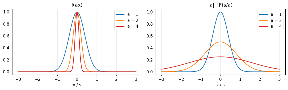
If f(x) has transform F(s) then f(ax) has transform |a|^{-1}F(s/a). Proof by the substitution x'=ax (Bracewell, p. 108). The modulus counteracts the interchange of limits when a<0.

Compress one axis and the other expands, with area conserved

Compressing the time scale corresponds to expanding the frequency scale. But as one member expands horizontally the other not only contracts horizontally but also grows vertically so as to keep constant the area beneath it (Fig. 6.2, p. 109). Measured with the Gaussian and a=2: f(2x) has area 0.5; its transform is 0.5 high at 0; at s=0.3 it equals 0.4659, exactly \tfrac12e^{-\pi(0.15)^2}.

An expanded cosinusoid: the impulses shift, they do not shrink

A special case with periodic functions and impulses: expanding a cosinusoid simply shifts the impulses of the transform. This is not simply a compression of the s scale, for that would reduce the strength of the impulses (Fig. 6.3, pp. 109 to 110). Measured with a Gaussian window a=0.05: the peak of \cos2\pi(2x) at s=2 is 10 high and that of \cos2\pi(4x) at s=4 is also 10 high.

The symmetric version of the similarity theorem

If f(x) has transform F(s) then |a|^{1/2}f(ax) has transform |b|^{1/2}F(bs) with b=a^{-1}. As each function expands or contracts it also shrinks or grows vertically to compensate, so the integral of its square is maintained constant, as the power theorem will show (Fig. 6.4, p. 110). Measured: \int f^2 = 0.7071 and \int(|a|^{1/2}f(ax))^2 is also 0.7071 for a=2.

The addition theorem

If f and g have transforms F and G then f+g has transform F+G. The theorem reflects the suitability of the Fourier transform for linear problems. A corollary: af has transform aF for a constant a (pp. 110 to 111). Measured: the transform of e^{-\pi x^2}+2e^{-|x|} at s=0.3 is 1.6322, exactly the sum of the transforms.

The shift theorem

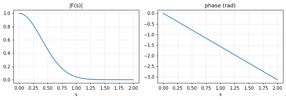
If f(x) has transform F(s) then f(x-a) has transform e^{-i2\pi as}F(s) (p. 111). Shifting a function by a in the positive direction changes no Fourier component in amplitude, so the changes in the transform are confined to phase. Measured with the Gaussian shifted by a=0.25 at s=0.3: magnitude 0.7537 (unchanged) and phase -27 degrees, exactly -2\pi as.

Why the phase is proportional to s

Each component is delayed in phase by an amount proportional to s: the higher the frequency, the greater the change in phase angle. This is because the absolute shift a occupies a greater fraction of the period s^{-1} at higher frequency. The phase delay is a/s^{-1} cycles or 2\pi as radians; the constant 2\pi a is the rate of change of phase with frequency (p. 111). Measured: the slope of the unwrapped phase against s is -1.5708 rad per unit of s, exactly -2\pi a.

A physical example: steering a beam with a prism

The shift theorem is self-evident in a chosen physical embodiment. Consider parallel monochromatic light falling normally on an aperture. To shift the diffracted beam through a small angle, one changes the angle of incidence by that amount. But that is simply a way of making the phase of the illumination change linearly across the aperture; another way is to insert a thin prism that injects delays proportional to the prism thickness at each point (pp. 111 to 112; chapter 13 returns to it).

Twist: shifting by a quarter twists the transform 90 degrees per unit of s

Take a function whose transform is real. Shifting it by \tfrac14 unit of x corresponds to a uniform twist of \pi/2 per unit of s; the plane containing F(s) is deformed into a helicoid (Fig. 6.6, pp. 112 to 113). Measured: the phase at s=1 is -90 degrees, at s=2 it is 180 degrees (or +180 after wrapping).

A sliding cosine: from real to imaginary

A small shift of a cosine leaves the real part of the transform almost intact but introduces an odd imaginary part. With further shift the imaginary part increases until at a shift of \pi/2 there is no real part left; then the real part reappears with opposite sign until at a shift of \pi both components have undergone a full reversal (Fig. 6.7, p. 113). The DFT coefficient at the cosine's frequency: 0.995 and -0.0998 (real, imaginary) for a phase shift of 0.1 rad; 0 and -1 for \pi/2; -1 and 0 for \pi.

Self-check, part 2

• If f(3x) is 3 times narrower, how does the transform change in width and height?
• What does shifting f by a do to |F| and to the phase?
• Why do a tilt of the beam and a prism both steer the beam?

Hints: 3 times wider, 1/3 as high; |F| unchanged, phase gets -2\pi as; because both make the phase change linearly across the aperture.

The modulation theorem

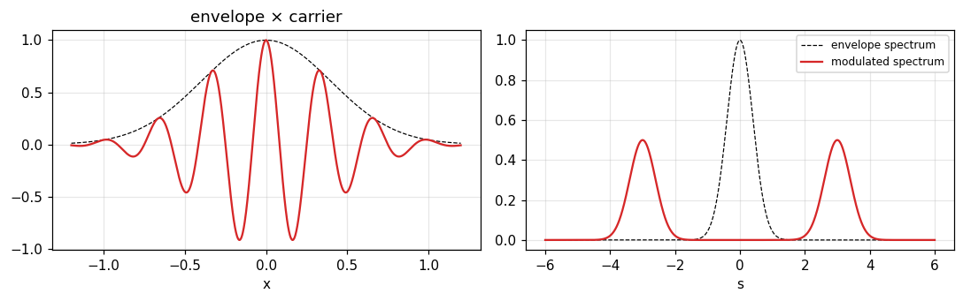
If f(x) has transform F(s) then f(x)\cos\omega x has transform \tfrac12F(s-\omega/2\pi)+\tfrac12F(s+\omega/2\pi) (Bracewell, pp. 113 to 114). The proof writes \cos\omega x through two complex exponentials and applies the shift theorem to the transform.

A special case of the convolution theorem

The new transform is the convolution of F(s) with \tfrac12\delta(s+\omega/2\pi)+\tfrac12\delta(s-\omega/2\pi). In radio and television a harmonic carrier is modulated by an envelope; the spectrum of the envelope separates into two parts, each of half the strength, shifted along the s axis by \pm\omega/2\pi (Fig. 6.8, p. 115). Measured: with a Gaussian envelope and carrier f_0=3, the peak at s=3 is 0.5 high, exactly \tfrac12F(0).

A radio-frequency pulse: the spectrum is two sinc functions

The pulse \Pi(x/X)\cos2\pi fx has spectrum \tfrac12X\{\text{sinc}[X(s+f)]+\text{sinc}[X(s-f)]\} (problem 8, p. 131). With X=10, f=1: at s=1 the spectrum equals 5; at s=1.05 it equals 3.2607, by both numerical integration and the formula.

An amplitude-modulated pulse: carrier and two sidebands

The pulse \Pi(x/X)(1+M\cos2\pi Fx)\cos2\pi fx has a spectrum with a carrier \tfrac12X\text{sinc} at \pm f and four sidebands of strength \tfrac14MX at \pm f\pm F (problem 9, p. 132). With X=200, f=50, F=5, M=0.6: carrier 100, sideband 30, ratio 0.3, exactly M/2.

The convolution theorem

If f has transform F and g has transform G then f*g has transform FG: convolution of two functions means multiplication of their transforms (p. 117). Proof: interchange the order of integration and use the shift theorem.

Linearity plus invariance decides when it applies

A train slowly crosses a bridge: the load at x is f(x) and the deflection at x is h(x). Since the members are not pushed beyond the regime where stress is proportional to strain, the deflection is a duly weighted linear combination of the load. But as the train moves on, the deflection pattern does not move with it unchanged, so it is not a convolution. Linearity combined with x-shift invariance is what makes Fourier analysis useful; it is also the condition for harmonic inputs to give harmonic outputs of unaltered frequency (p. 115).

Four statements in words

1. The transform of a convolution is the product of the transforms.
2. The transform of a product is the convolution of the transforms.
3. The convolution of two functions is the transform of the product of their transforms.
4. The product of two functions is the transform of the convolution of their transforms.

With bar notation: \overline{f*g}=\bar f\bar g and \overline{fg}=\bar f*\bar g; also f*g*h\supset FGH (p. 117).

Three checks often used

• The area under a convolution equals the product of the areas: \int(f*g)=\int f\int g.
• The abscissas of the centres of gravity add: \langle x\rangle_{f*g}=\langle x\rangle_f+\langle x\rangle_g.
• The second moments add if \langle x\rangle_f or \langle x\rangle_g is 0, i.e. the variances add (p. 118).

Measured with f=e^{-x}H(x) and g=\Pi: area 1, centre of gravity 1, variance 1.0833 =1+1/12.

The twenty forms of the theorem

Allowing for complex conjugates and sign reversals of the variables, there are 20 versions of the convolution theorem that are constantly needed. Bracewell lists 10 abbreviated forms (pp. 118 to 119), such as f*g\supset FG, f*g(-)\supset FG(-), f*g^*(-)\supset FG^*, f^*(-)*g^*(-)\supset F^*G^*. The notebook checks 9 of these forms with the DFT on complex sequences, comparing the direct sum with the product of DFTs.

The convolution theorem numerically: two ways

For two complex sequences of length 64, the circular convolution computed by the direct sum and by \text{IFFT}(F\cdot G) differ by at most 1.5e-14. That is why the FFT speeds up convolution (modules 3 and 14).

Self-check, part 3

• What does multiplying by \cos2\pi f_0x do to the spectrum, and how strong is each replica?
• Why is the bridge deflection as the train moves not a convolution?
• What is the variance of f*g if f has variance 2 and g has variance 3 (unit areas)?

Hints: two half-strength replicas shifted by \pm f_0; because it lacks x-invariance; 5.

Rayleigh's theorem

The integral of the squared modulus of a function equals the integral of the squared modulus of its spectrum (Bracewell, p. 119). It corresponds to Parseval's theorem for Fourier series and was first used by Rayleigh in 1889 in his study of black-body radiation; each integral represents the energy of a system, one taken over all values of a coordinate, the other over all spectral components (Fig. 6.9, pp. 119 to 120).

Conditions and names

In mathematical circles the theorem is called Plancherel's theorem (Titchmarsh, 1924) after M. Plancherel, who in 1910 established conditions under which it is true: it holds if both integrals exist. More recently Carleman showed it is true if one of the integrals exists. Rayleigh simply assumed the integrals existed (p. 120).

Numerical test: two examples

For the Gaussian e^{-\pi x^2}: \int f^2 = 0.7071 and \int|F|^2 = 0.7071. For e^{-x}H(x): \int|f|^2 = 0.5 and \int|F|^2ds=\int ds/(1+4\pi^2s^2) = 0.5. The same numbers by two independent computations.

The power theorem

More general than Rayleigh's, for a product of two functions: \int f\,g^*dx=\int F\,G^*ds. Each side is energy or power computed two ways. In the first, instantaneous power is the product of a pair of canonically conjugate variables (electric and magnetic fields, voltage and current, force and velocity) integrated over time or space. In the second, the spectral components are multiplied and integrated over the whole spectrum (p. 120).

Numerical test: two shifted Gaussians

For f=e^{-\pi(x+0.3)^2} and g=e^{-\pi(x-1)^2}: \int fg\,dx = 0.0497 and \int FG^*ds = 0.0497, equal. Here f and g are real so F and G are complex.

For real f, g: real and imaginary parts suffice

If f and g are real then F and G are Hermitian: real parts even, imaginary parts odd. The odd terms do not contribute to the infinite integral, so \int fg\,dx=\int[\text{Re}F\,\text{Re}G+\text{Im}F\,\text{Im}G]ds (Fig. 6.11, p. 121). In the example above the two parts integrate to 0.1886 and -0.1389, summing to 0.0497.

The autocorrelation theorem

The autocorrelation \int f^*(u)f(u+x)du of f has transform |F(s)|^2. In communications this reads: the autocorrelation function of a signal is the Fourier transform of its power spectrum; Fig. 6.12 illustrates it (p. 122). The distinguishing feature against self-convolution: information about the phase of F(s) is entirely missing from |F|^2, just as the autocorrelation contains no information about the phases of the Fourier components (module 3, p. 45).

Numerical test: \Pi\star\Pi=\Lambda and the \text{sinc}^2 spectrum

The autocorrelation of \Pi is \Lambda, with transform 0.7368 at s=0.3, exactly \text{sinc}^2(0.3)=|\text{sinc}\,0.3|^2. For the Gaussian, the normalised autocorrelation e^{-\pi x^2/2} has transform \sqrt2e^{-2\pi s^2} with integral 1: the normalised power spectrum whose infinite integral is unity (the book's exercise, p. 122).

The limit C(x) and the power spectrum; Wiener's theorem

For signals that run on, the normalised autocorrelations \gamma_X(x) may tend to a limit C(x), and then the normalised power spectrum of a segment of length X tends to a limiting form: C(x)\supset|\Phi_\infty(s)|^2. The corresponding theorem for signals that do not tend to zero is sometimes called Wiener's theorem (1949) (pp. 122 to 123). For example f=\cos ax has C=\cos ax and the spectrum is the impulse pair \tfrac12\delta(s\pm a/2\pi). Measured over a 10 s segment of \cos2\pi(5t): the fraction of power at +5 Hz and at -5 Hz is 0.5 on each side.

Self-check, part 4

• Rayleigh holds for e^{-x}H(x): what do the two sides equal?
• Why does the power theorem need the conjugate g^*?
• Can the signal be recovered from its autocorrelation?

Hints: ½; so both sides give positive energy for complex functions; no, because the phase is lost.

The derivative theorem

If f(x) has transform F(s) then f'(x) has transform i2\pi sF(s) (Bracewell, p. 124). Proof: write the derivative as the limit of a difference quotient and use the shift and addition theorems. Measured with f=e^{-\pi x^2}: the transform of f' at s=0.3 has magnitude 1.4207, exactly 2\pi s\,e^{-\pi s^2}.

Differentiation enhances high frequencies

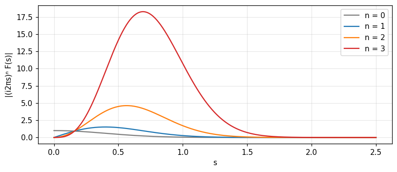
Multiplying by i2\pi s means differentiation enhances the higher frequencies, attenuates the lower frequencies and suppresses any zero-frequency component (Figs. 6.13 and 6.14, p. 125). Repeated application multiplies by (i2\pi s)^n: the maximum of |(2\pi s)^ne^{-\pi s^2}| lies at 0.3989 (n=1), 0.5642 (n=2), 0.691 (n=3), shifting up in frequency, exactly \sqrt{n/2\pi}.

When the derivative has infinite discontinuities: impulses step in

It frequently happens that multiplication by i2\pi s makes the integral of |i2\pi sF(s)| diverge; correspondingly f'(x) exhibits infinite discontinuities. Such situations are accommodated by the impulse symbol and its derivatives (p. 125). Measured with the decaying step e^{-\varepsilon x}H(x): the transform of the derivative is i2\pi s/(\varepsilon+i2\pi s), which differs from 1 (the transform of \delta) by only 3.2e-04 for \varepsilon=10^{-3} and s=0.5.

The derivative of a convolution

From the derivative theorem together with the convolution theorem: if h=f*g then h'=f'*g=f*g': the derivative of a convolution is the convolution of either function with the derivative of the other (p. 126). In impulse notation h=\delta*h, so h'=\delta'*h=(\delta'*f)*g=f'*g. The formulas are mostly of theoretical value, such as deducing the uncertainty relation and the filter response from the impulse and step responses.

Numerical test: the response through the step response

For an RC circuit (h=e^{-t}H(t), step response s(t)=1-e^{-t}) and a smoothly switched-on input x(t)=\sin(2\pi t), the response y=x*h equals x'*s: the largest deviation is 5.3e-04. Knowing the step response is enough to compute the response to any differentiable input.

The transform of a generalized function

Let p(x) be a generalized function defined by the sequence p_\tau; transform the members to P_\tau(s). From the energy theorem the sequence P_\tau is regular so it defines a generalized function P(s), the Fourier transform of p, with \int PF\,ds=\int p(x)f(-x)dx for every test function (p. 127). Measured with p=\delta(x-a), a=0.5: \int e^{-i2\pi as}e^{-\pi s^2}ds = 0.4559, exactly e^{-\pi a^2}.

Multiplying by polynomials, and why there is no product of two generalized functions

If \phi(x) has derivatives of all orders but grows no faster than a power (a polynomial, but not e^x or \log x) then \phi p is still a generalized function. But nothing is introduced that could be called the product of two generalized functions: the product of two defining sequences is not necessarily regular (pp. 127 to 128). So [\delta(x)]^2 has no meaning, and the best power theorem that can be proved is \int PF\,ds=\int pf(-x)dx (p. 129).

Rigorous proofs: similarity with shift, and the derivative

The short "derivations" in the chapter are useful while learning but do not qualify as strict proofs (as in Lighthill, 1958). For generalized functions, similarity and shift are proved together: p(ax+b)\supset|a|^{-1}e^{i2\pi bs/a}P(s/a). The derivative theorem: the transform of p_\tau' is i2\pi sP_\tau so that of p' is i2\pi sP (pp. 128 to 129). Measured with the Gaussian, a=2, b=0.3, s=0.4: magnitude 0.441, phase 21.6 degrees, by numerical integration and the formula.

Two dimensions

All the above theorems generalise readily to two dimensions. Rotation and shear, which do not arise in one dimension, are associated with new basic theorems, circular symmetry introduces important special cases, and the affine theorem for functions of the form f(ax+by+c,\,dx+ey+f) has rich implications for graphics (Bracewell et al. 1993, Bracewell 1994) (p. 129).

Table 6.1: the theorems

Selected problems: trapezoid, \text{sinc}^4, xe^{-\pi x^2} and the integral theorem

Problem 10 (p. 132): the trapezoid f=2\Lambda(x/2)-\Lambda(x) has F=\text{sinc}^2s\,(1+2\cos2\pi s), equal to 0.2814 at s=0.3. Problem 17 (p. 133): by Rayleigh, \int\text{sinc}^4x\,dx=\int\Lambda^2=\tfrac23 = 0.6667. Problem 21: the transform of xe^{-\pi x^2} is -is\,e^{-\pi s^2}, magnitude 0.2261 at 0.3. Problems 19 and 20: the transform of the indefinite integral \int_{-\infty}^xf is F(s)/(i2\pi s) plus \tfrac12F(0)\delta(s) (the forgotten term): measured deviation 1.2e-17 when checking \text{FT}[H*f-H]=(F-1)/(i2\pi s).

Self-check, part 5

• What is the transform of f''?
• Why is h'=f'*g=f*g'?
• Why is "the transform of \int f is F/i2\pi s" not the whole story?

Hints: (i2\pi s)^2F; from the derivative and convolution theorems; the term \tfrac12F(0)\delta(s) (the DC component) is missing.

Takeaways

• Similarity inverts the two axes and conserves area; shift only multiplies by e^{-i2\pi as}, keeping |F|.
• Modulation gives two half-strength replicas shifted \pm f_0; convolution is multiplication of spectra and vice versa.
• Rayleigh and power connect energy in x with s; autocorrelation \supset|F|^2 and loses phase.
• Differentiation is multiplication by i2\pi s; the derivative of a convolution moves onto one factor.
• The theorems extend to generalized functions, but there is no product of two generalized functions.

References

R. N. Bracewell, The Fourier Transform and Its Applications, 3rd ed., McGraw-Hill, 2000, chapter 6 (pp. 105 to 135).
The content was written with AI assistance (Claude) and then checked. Every number is produced by a Jupyter notebook and cross-checked by two independent methods; page citations come from the OCR text of the two source books. Mistakes may remain, so please report them.
R. N. Bracewell, The Fourier Transform and Its Applications, 3rd ed., McGraw-Hill, 2000.
M. Barkat, Signal Detection and Estimation, 2nd ed., Artech House, 2005.
This site only summarises, explains and checks numbers; please read the original books through a library or the publisher.
Contribute
Report errors, suggest modules or translations in the GitHub repository, and fork or clone it for your own study. Please credit the source when sharing.