The two domains: a function and its transform

The two domains: a function and its transform

• State and use the pairs of properties: area and central ordinate, nth moment and nth derivative at the origin, centroid, variance.
• Relate the smoothness of a function to the decay rate of its transform (log-log slope, decibels per octave).
• Compute equivalent width, autocorrelation width and mean-square width, and understand the uncertainty relation.
• Use finite differences and running means, and explain the central-limit theorem through transforms.
• Use the inequalities: upper bounds on ordinate and slope, and Schwarz's.

Use the buttons, the dots or the ← → keys to move between slides.

Two domains

We may think of functions and their transforms as occupying two domains, sometimes called the upper and the lower, as if functions circulated at ground level and their transforms in the underworld (Doetsch, 1943). Each function is accompanied by a counterpart, a shadow in the other domain, associated uniquely with it through the Fourier transform and changing as the function changes. In the illustrations functions are on the left and transforms on the right (Bracewell, p. 151).

The theorems are pairs of operations

The earlier theorems are a list of pairs of simultaneous operations, one in the function domain and one in the transform domain. Compression of the abscissas in the function domain means expansion of the abscissas and contraction of the ordinates in the transform domain; translation means a twisting; convolution means multiplication. We now consider pairs of corresponding properties: the area under a function and the central ordinate of its transform are such a pair (pp. 151 to 152). The purpose: when only a feature of a function is needed, cross to the other domain and read the answer directly.

The definite integral

The definite integral of a function from -\infty to \infty equals the value of its transform at the origin, since F(0)=\int f(x)e^{0}dx (p. 152). By symmetry the area under the transform equals f(0). Measured with f=e^{-x}H(x): the area 1 equals F(0) = 1, and the area under F equals 0.5, the mean of f on the two sides of the jump at 0.

Consequence: any operation that preserves area

Any operation on f(x) that leaves its area unchanged, say translation, leaves the central ordinate of the transform unchanged; for translation this agrees with the shift theorem since e^{-i2\pi as}F(s) at s=0 equals F(0). A harder example: split f at x=0 into two halves and push them apart by 2a, giving f(x-a)H(x-a)+f(x+a)H(-x-a). The area is unchanged so the central ordinate of the transform is too; since the central ordinate of the function is now zero, the area of the transform must be zero (p. 152). Measured with f=e^{-|x|}, a=0.5: the area is 2, and the area of the transform is 0.

The first moment

By analogy with mass distribution along a line, the first moment about the origin is \int xf(x)dx. Theorem: the first moment equals -(2\pi i)^{-1} times the slope of F(s) at s=0 (pp. 153 to 154). It follows from the derivative theorem: \int(-i2\pi x)f(x)e^{-i2\pi xs}dx=F'(s). Measured with f=e^{-x}H(x): \int xf= 1, and F'(0)/(-2\pi i) = 1.

The special case of zero first moment

A function whose first moment is zero has a transform with zero slope at its origin, and conversely. Furthermore, if a function has zero slope at the origin and is not zero there, its transform has its centre of gravity at the origin (p. 155). Measured: the even Gaussian has first moment 0 and its transform has slope 0 at the origin.

The centroid

The centroid \langle x\rangle is the point such that the area times \langle x\rangle equals the first moment; it tells where a function is mainly concentrated, or the epoch of a signal pulse (p. 155). From the preceding sections \langle x\rangle=F'(0)/(-2\pi iF(0)): the abscissa of the centroid is the central slope over the central ordinate of the transform, times -(2\pi i)^{-1}. If the area is zero, \langle x\rangle becomes infinite (p. 156). Measured with f=xe^{-x}H(x) (Table 8.4): F=(1+i2\pi s)^{-2}, centroid 2 by integration and 2 by F'(0)/(-2\pi iF(0)).

The moment of inertia (second moment)

The second moment \int x^2f\,dx equals (4\pi^2)^{-1} times the downward curvature of the transform at the origin: \int x^2f\,dx=-F''(0)/4\pi^2 (pp. 156 to 157). A function with a high second moment has a transform that is strongly curved at the origin; because of the factor x^2 the moment is sensitive to f at large x, and what happens at large x is reflected in the behaviour of the transform at the origin of s. If the second moment is infinite the slope of the transform jumps abruptly at the origin (Fig. 8.5). Measured with f=xe^{-x}H(x): \int x^2f= 6, and -F''(0)/4\pi^2 = 6.

The nth moment and existence

The nth moment equals (-2\pi i)^{-n} times the nth derivative of F at the origin, provided the moment exists (p. 157). If f behaves as |x|^{-m} for large |x| then only the first [m]-1 moments exist and the transform has a higher-order discontinuity at the origin; if the Mth derivative of F is impulsive the Mth moment is infinite (p. 158). Measured with f=e^{-x}H(x), n!: the moments of order 2, 3, 4 equal 2, 6, 24 both by integration and from derivatives of F (a contour integral around the origin).

Self-check, part 1

• Why does pushing the two halves of f apart make the area of the transform zero?
• When is the centroid undefined?
• Why is the second moment sensitive to the behaviour of f at large x?

Hints: because the central ordinate of the function is zero; when the area is zero; because of the factor x^2.

The mean-square abscissa

\langle x^2\rangle is the mean of x^2 weighted by f(x), and by the previous results \langle x^2\rangle=\dfrac{-F''(0)}{4\pi^2F(0)} (p. 158). In dynamics \langle x^2\rangle is the square of the radius of gyration of a rod of mass density f; in statistics, for a frequency distribution function, it is an important concept and F is the "characteristic function" (p. 158). For f=xe^{-x}H(x) the value is 6 (Table 8.4).

Additivity under convolution

The mean-square abscissa of f*g equals the sum for f and g provided that f (or g) has its centroid at the origin. This is a quantitative expression of the smoothing-out or diffusing effect of convolution. Derivation: (FG)''=F''G+2F'G'+FG'', so in general (pp. 158 to 159):

Measured with f=xe^{-x}H (centroid 2, \langle x^2\rangle=6) and g=e^{-x}H (centroid 1, \langle x^2\rangle=2): \langle x^2\rangle_{f*g} = 11.994 equals 6+2+2\cdot2\cdot1; the convolution measured on a grid gives the same number.

A displaced axis: the parallel-axis theorem

Take g(x)=\delta(x-a), for which \langle x^2\rangle_g=a^2; we obtain the familiar theorem on the moment of inertia of a mass about an axis not through its centre of gravity: if f has its origin at its centroid, \langle x^2\rangle_{f*\delta_a}=\langle x^2\rangle_f+a^2 (p. 159). Measured with the triangle \Lambda (\langle x^2\rangle=1/6) shifted by a=2: 4.1667 =1/6+4.

Radius of gyration and variance

The radius of gyration is the square root of the mean-square abscissa, convenient for having the same dimensions as x, though the properties (additivity, curvature) are simpler in terms of \langle x^2\rangle (p. 159). The variance \sigma^2=\langle(x-\langle x\rangle)^2\rangle=\langle x^2\rangle-\langle x\rangle^2 is the mean-square deviation from the centroid; it equals \langle x^2\rangle when the origin is at the centroid. The variance of f*g equals the sum of the variances (p. 160). Measured with f=xe^{-x}H and \Lambda: \sigma_f^2 = 2, \sigma_\Lambda^2 = 0.1667, and the convolution has variance 2.1667.

Smoothness and compactness

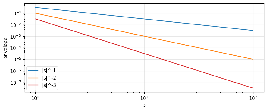
The smoother a function is, as measured by the number of continuous derivatives it possesses, the more compact its transform, i.e. the faster it dies away with increasing s. If a function and its first n-1 derivatives are continuous its transform dies away at least as rapidly as |s|^{-(n+1)}; in short, if the kth derivative becomes impulsive the transform behaves as |s|^{-k} at infinity (pp. 160 to 161). That is why \text{sinc}^2x dies away much faster than \text{sinc}\,x, associated with the transform \Lambda being smoother than \Pi (Fig. 8.6).

Numerical test: the log-log slope

Measured by numerical integration at half-integer points s=10.5 and 20.5: the rectangle (the function itself jumps) gives slope -1; the triangle (first derivative jumps, second is impulsive) gives -2; the piecewise parabolic pulse \Pi*\Pi*\Pi (third derivative impulsive) gives -3. Each further convolution with \Pi steepens the slope by one unit.

Decibels per octave

A function with corners but no jumps (discontinuous derivative) has a transform dying as s^{-2} and a power spectrum as s^{-4}; in electric-circuit language that is attenuation at 12 decibels per octave or 40 decibels per decade (p. 163). On a log-log plot a function varying as s^{-2} is a straight line of slope -2; logarithmic units (octave, decade, decibel, neper) let the dimensionless slope be stated in expressive units. Measured: 20\log_{10}2\times2 = 12 dB per octave, and 40 dB per decade for s^{-2}.

Intermediate discontinuities and smoothness under convolution

Some discontinuities have severity between a jump and a corner: a corner where a function changes slope from horizontal to vertical ranks midway between simple corners and simple jumps (Table 8.2, pp. 164 to 165). \delta(x) and x^{-1} have the same kind of infinity at 0, and the weakest infinite discontinuity, \log x, is equivalent to a simple jump. On convolution: if f has smoothness of order m and g of order n then f*g has smoothness m+n, since F\sim s^{-m}, G\sim s^{-n}, FG\sim s^{-(m+n)} (pp. 162 to 163). Smoothness adds under convolution just as \sigma^2 does. But smoothness so measured does not always match qualitative ideas: \Lambda convolved with a very narrow Gaussian is infinitely smooth yet only its tiny corners are rounded, so the ride is as rough as before (p. 163).

Self-check, part 2

• What is the variance of f*g if \sigma_f^2=2 and \sigma_g^2=3?
• How does the transform decay if the third derivative of the function is impulsive?
• 12 dB per octave corresponds to which power of s?

Hints: 5; as |s|^{-3}; s^{-2} (amplitude).

Equivalent width

A convenient measure of width is the area divided by the central ordinate: W_f=\int f\,dx/f(0). In other words it is the width of the rectangle whose height equals the central ordinate and whose area equals that of the function (Fig. 8.8, pp. 164 to 165). In spectroscopy the equivalent width of a spectral line is the width of a rectangular profile with the same central intensity and the same area; in antenna theory the effective beamwidth has the character of an equivalent width (p. 165).

Some examples

If f(0)=0 the equivalent width does not exist. Measured (numerical integration): e^{-|x|} has W = 2; the Lorentzian 1/(1+x^2) has W = 3.1416 (=\pi); \Lambda has 1; the Gaussian e^{-\pi x^2} has 1 (Table 8.3).

The reciprocity theorem

The equivalent width of a function equals the reciprocal of the equivalent width of its transform: W_fW_F=1 whenever both exist (p. 167). The theorem is reminiscent of the similarity theorem, which however is restricted to functions of a given shape; here we know which quantity behaves reciprocally, and unlike functions can be ranked by it. Proof: W_F=\int F\,ds/F(0)=f(0)/\int f\,dx. Measured: W_fW_F = 1 for e^{-|x|} (with W_F = 0.5) and 1 for the Lorentzian (with W_F = 0.3183).

Limits of equivalent width

Equivalent width is not always the best measure. For the bandwidth of a filter or the beamwidth of an antenna the "width to half power" is common, and by that measure the second example of Fig. 8.9 is narrower, agreeing with experience (p. 167). A paradox: a localised turbulent motion spreads outward in space while its spectrum spreads to higher wavenumbers; here equivalent width is the wrong measure. The effective solid angle of an antenna pattern, equal to 4\pi over directivity, is the equivalent width generalised to two dimensions (p. 167).

Autocorrelation width

The autocorrelation width is the equivalent width of the autocorrelation function: W_{f\star f}=\dfrac{\int f\star f\,dx}{(f\star f)(0)}=\dfrac{|\int f\,dx|^2}{\int|f|^2dx} (p. 170). It does not necessarily refer to concentration about the origin: two functions with the same autocorrelation (Fig. 8.10) have the same autocorrelation width but different equivalent widths. For a rectangular pulse the equivalent width can break down simply from displacement because the central ordinate falls to zero; autocorrelation width avoids this since the autocorrelation is maximal at the origin, never zero. Measured: \Pi shifted by 3 units has W_{f\star f} = 1 as before the shift, while its f(0) is 0.

Relation to the power spectrum

From the reciprocity, the autocorrelation width of a function is the reciprocal of the equivalent width of its power spectrum |F|^2; and the reciprocal of the autocorrelation width of the transform is the equivalent width of |f|^2 (p. 170). So the idea breaks down when |F|^2 has a zero central ordinate, i.e. when the function has no d.c. component, as for wave packets (p. 170). Measured with e^{-|x|}: W_{f\star f} = 4, and 1/W_{|F|^2} = 4, the same result by two calculations.

Strengths and limits of autocorrelation width

Two functions with the same power spectrum, whose spectral components are slid into any relative phase, have the same autocorrelation. So W_{f\star f} (1) copes with displacement of the function from the origin and (2) copes with internal phase interference that gives a small central ordinate. But of two functions with the same power spectrum, one can be narrow and the other wide: Fresnel diffraction fields on planes parallel to an illuminated aperture have the same autocorrelation while the illuminated width grows with distance (p. 171). For white noise passed through a filter and rectified, the average interval between effectively independent output values is inversely proportional to the autocorrelation width of the power pass characteristic (p. 171). Autocorrelation width is also invariant under shuffling.

Self-check, part 3

• What are W_f and W_F for e^{-|x|}?
• Why does \Pi(x-3) have an autocorrelation width but no equivalent width?
• When is the autocorrelation width undefined?

Hints: 2 and 1/2; because f(0)=0 while the autocorrelation peaks at the origin; when the function has zero area.

When the earlier measures fail

The equivalent width and concentration just described do not fill all needs, so other measures of width are also used. The mean-square value \langle x^2\rangle=\int x^2f/\int f is widely appropriate, as is the variance for functions not centred on the origin: \langle(x-\langle x\rangle)^2\rangle=\langle x^2\rangle-\langle x\rangle^2=\dfrac{-F''(0)}{4\pi^2F(0)}+\dfrac{1}{4\pi^2}\left[\dfrac{F'(0)}{F(0)}\right]^2 (p. 171). These measures break down when the area of the function is zero and are therefore inappropriate for oscillatory signals or wave packets (p. 172).

The variance of the squared modulus

To cope, we think in terms of the energy density |f|^2: the centroid and variance of the energy distribution, called the variance of the squared modulus, (\Delta x)^2=\dfrac{\int(x-\bar x)^2|f|^2dx}{\int|f|^2dx} (p. 172). This may seem an elaborate expression for the simple idea of the duration or bandwidth of a signal packet, but it behaves more reasonably for many purposes. However |f|^2 may not have finite variance: \text{sinc}\,x and (x^2+1)^{-1}, two concentrated peaked functions with reasonable equivalent and autocorrelation widths, show up as infinitely broad on a variance basis (p. 172). Caution is therefore needed before assuming that widths based on variance relate to intuitive ideas of width.

An upper limit to the ordinate

How large can a function become? From f(x)=\int F(s)e^{i2\pi xs}ds we get |f(x)|\le\int|F(s)|ds (p. 174). On the complex plane of f(x) the Fourier integral at a given x is an arc whose length \int|F|ds does not depend on x; the maximum |f| can reach is when the arc straightens, i.e. all components come into phase. Measured with the shifted Gaussian f(x)=e^{-\pi(x-0.5)^2}: |f(0)| = 0.4559 while \int|F|ds = 1; equality is reached at x=0.5, where all components are in phase, with f(0.5) = 1.

An upper limit to the slope

The component F(s)e^{i2\pi xs}ds has slope i2\pi sF(s)e^{i2\pi xs}ds, and considering the possibility of all components reaching maximum slope together: |f'(x)|\le2\pi\int|sF(s)|ds (p. 176). Both inequalities stem from the geometric fact that an arc joining two points is at least as long as the chord, i.e. two sides of a triangle together are at least the third, |A+B|\le|A|+|B| (p. 176). Measured with the Gaussian: \max|f'| = 1.5203 and the bound 2.

Schwarz's inequality

For two real functions f and g on a\le x\le b: \left[\int fg\,dx\right]^2\le\int f^2dx\int g^2dx. The general form for complex functions: \left|\int(F^*G+FG^*)dx\right|^2\le4\int FF^*dx\int GG^*dx (p. 176). Proof: consider 0\le\int(F+\epsilon G)(F+\epsilon G)^*dx, a quadratic in real \epsilon, which has no real zero if b^2-4ac\le0. It is the analogue of the vector inequality \mathbf A\cdot\mathbf B\le AB. Measured with f=\Lambda and g=e^{-|x|}: (\int fg)^2 = 0.5413 \le\int f^2\int g^2 = 0.6667.

The uncertainty relation: statement

The bandwidth-duration product of a signal cannot be less than a certain minimum; it is a mathematical phenomenon bound up with the interdependence of time and frequency, which prevents arbitrary specification of both function and spectrum. A finite area of the time-frequency plane can contain only a finite number of independent data (p. 177). For equivalent widths W_fW_F=1 always; for autocorrelation widths the product is also determined; but for mean-square widths the product is not constant and can range from zero to infinity (p. 177). With the variance (\Delta x)^2 of |f|^2 and (\Delta s)^2 of |F|^2:

The proof

Use the theorem \int f'f'^*dx=4\pi^2\int s^2FF^*ds (derivative theorem with Rayleigh), Schwarz, and integration by parts \int xf\,f'dx=-\tfrac12\int f^2dx (pp. 177 to 178). With f and F centred on their centroids, (\Delta x)^2(\Delta s)^2=\dfrac{\int x^2ff^*dx\ \int s^2FF^*ds}{\int ff^*dx\ \int FF^*ds}\ge\dfrac{1}{16\pi^2}, i.e. \Delta x\,\Delta s\ge\dfrac1{4\pi}. Equality only when f'\propto xf, i.e. a Gaussian.

Example: the Gaussian attains the minimum, the two-sided exponential does not

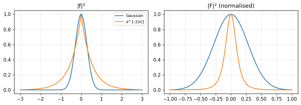
For f=\exp(-\pi a^2x^2), |f|^2 has variance 1/4\pi a^2 and |F|^2 has variance a^2/4\pi, so \Delta x\,\Delta s=1/4\pi, exactly the minimum (p. 179). Measured (a=1): 0.0796, both by direct integration and by the formula. For f=e^{-|x|}: \Delta x= 0.7071, \Delta s= 0.1592, product 0.1125, larger than the minimum 0.0796 by a factor of about 1.41.

Physics: a radar pulse and ways to measure bandwidth

Bracewell considers a radar transmitter emitting a 1-microsecond pulse at 10,000 MHz; the uncertainty relation gives \Delta t\,\Delta f\ge1/4\pi, i.e. \Delta f\ge 79577 Hz for \Delta t=1\ \mus. But experience with receivers shows a bandwidth of 1 MHz is the optimum choice for detecting such a pulse, so the relation is only a lower limit, far from practice. He also points out that the product \Delta t\,Df, with Df the width of the positive-frequency power spectrum (f>0 only), is not subject to the lower limit 1/4\pi (Uffink and Hilgevoord, 1985, 1988): for example s(t)=\exp(-\alpha t^2)\cos2\pi f_0t gives a product 0.400\times(1/4\pi), below the quantum limit (p. 180). Lesson: pick the right definition of width before stating a limit.

Self-check, part 4

• Which function shape attains the minimum \Delta x\,\Delta s=1/4\pi?
• When does the bound |f|\le\int|F| reach equality?
• Why is the variance of |f|^2 infinite for f=\text{sinc}\,x?

Hints: the Gaussian; when all components are in phase at that x; because \text{sinc}^2x only decays as x^{-2} so x^2\text{sinc}^2x is not integrable.

The finite difference

The finite difference of f(x) over the interval a is \Delta_af(x)=f(x+\tfrac12a)-f(x-\tfrac12a) (Bracewell, p. 180). It is often met with functions tabulated at discrete intervals but can also be taken for functions defined for all x. When a is small, \Delta_af is small but approaches proportionality to the derivative; when a is large, \Delta_af may separate into a displaced f(x) followed by an inverted one (Figs. 8.15 and 8.16). It is a convolution: \Delta_af=\big[\delta(x+\tfrac a2)-\delta(x-\tfrac a2)\big]*f, the odd impulse pair (p. 182).

The transform of a difference

The transform of the odd impulse pair is known, so by the convolution theorem the transform of \Delta_af is 2i\sin(\pi as)F(s) (p. 183). Differencing over a wide interval multiplies the transform by a high-frequency sinusoid; over a small interval, by a low-frequency sinusoid; for an interval shorter than the finest structure the sinusoid is effectively a linear function of s. Connection with differentiation: \lim_{a\to0}\dfrac{2i\sin\pi as}{a}=i2\pi s. Measured with the Gaussian, a=0.5, s=0.3: |\text{FT}[\Delta_af]| = 0.6844, equal to 2\sin(\pi as)F (numerical integration and formula). With a=10^{-3}, \Delta_af/a differs from f' by only 1.5e-07 (relative).

The second difference

The second difference \Delta_a^2f(x)=f(x+a)-2f(x)+f(x-a) is the difference of the difference, corresponding to two multiplications by 2i\sin\pi as, so its transform is -4\sin^2(\pi as)F(s). Geometrically the first difference is proportional to the average slope and the second to the average curvature over finite intervals (Fig. 8.19, p. 184). Measured at the same point: magnitude 0.6214.

Running means

In reducing meteorological data such as rainfall, unimportant day-to-day fluctuations are smoothed out with running means to reveal the seasonal trend. The running mean of f over the interval a is a^{-1}\Pi(x/a)*f(x) (pp. 184 to 185). Since the transform of a^{-1}\Pi(x/a) is \text{sinc}\,as, the transform of the running mean is \text{sinc}(as)F(s): taking running means corresponds to multiplication by \text{sinc}\,as. Measured with the Gaussian, a=1, s=0.3: the running mean computed with the error function and then transformed gives 0.647, equal to \text{sinc}(as)F.

Higher-order running means

The second-order running mean (applied twice) has transform \text{sinc}^2as\,F(s), and since \text{sinc}^2as is the transform of a^{-1}\Lambda(x/a) it is a triangle-weighted running mean. In general n applications give \text{sinc}^nas (Fig. 8.20, p. 186). Measured: \text{sinc}^2(as)F at s=0.3 is 0.5554. As a\to0, \text{sinc}\,as\to1 (the running mean tends to the original); as a\to\infty, \text{sinc}\,as\to a^{-1}\delta(s) (only the global mean survives).

The central-limit theorem

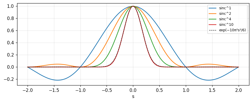
If a large number of functions are convolved, the result may be very smooth and, as the number increases indefinitely, may approach Gaussian form; the rigorous statement is the central-limit theorem (p. 186). Example: near s=0, \text{sinc}\,s\approx1-\pi^2s^2/6 so the nth profile is approximated by (1-\pi^2s^2/6)^n\to e^{-n\pi^2s^2/6}, a Gaussian that keeps narrowing (width varying as n^{-1/2}); its inverse transform is a Gaussian that keeps widening, its variance growing in proportion to n, a consequence of variances adding under convolution. Measured: n=10, s=0.2: \text{sinc}^{10}(0.2) = 0.5133 and the Gaussian 0.5179.

Numerical test: sums of uniform distributions

Convolving n unit rectangles: variance n/12 (adding) and excess kurtosis -6/5n tending to 0, the Gaussian signature. Measured with n=4: variance 0.3333 and excess kurtosis -0.3. Bracewell also suggests trying serial products such as \{1\ 1\}^{*n}: with n=20 the central coefficient is 0.1762 (binomial) against the Gaussian 0.1784.

Conditions of applicability

The essential thing is that the transform of each function should have a "humped" behaviour at the origin: a-bs^2. The coefficient a must be nonzero and finite (no function may have zero area, or the product of transforms would be zero at s=0); b must be finite, occasionally zero is fine. No factor should resemble \Lambda(s) at the origin since it would leave a permanent corner (p. 188). In the x domain: 0<\int f<\infty, \int xf finite (put the origin at the centroid), \int x^2f<\infty (p. 188). Not all functions go to Gaussian: \Pi(x)\sin2\pi x does not, but many unsymmetrical functions such as e^{-x}H(x) and discontinuous ones such as \Pi do. If one transform falls to zero at a finite s_1 the product has a zero too and cannot be exactly Gaussian, although in practice it may be indistinguishable (pp. 188 to 190).

Sampling and replication commute

If we replicate a function at integer interval X and then sample at unit interval, we get the same result as sampling first and then replicating the sample set at interval X (pp. 172 to 174). In operator form: X^{-1}\text{III}(x/X)*[\text{III}(x)\,f(x)]=\text{III}(x)\,[X^{-1}\text{III}(x/X)*f(x)]. It does not apply to functions like (1+x^2)^{-1} for which the replication sum does not exist. Measured with a wide Gaussian, X=4: the two orders differ by 0.0e+00.

Table 8.5: summary of correspondences

Self-check, part 5

• What is the transform of the second difference?
• Why may no function in the central-limit convolution have zero area?
• What does a second-order running mean correspond to?

Hints: -4\sin^2(\pi as)F; because the product of transforms would be zero at s=0; \text{sinc}^2as.

Takeaways

• The area equals the central ordinate; the nth moment is F^{(n)}(0)/(-2\pi i)^n; the centroid is the central slope over the central ordinate.
• Variance, mean-square and smoothness all add under convolution; a kth derivative that is impulsive makes the transform decay as |s|^{-k}.
• The equivalent width of a function is the reciprocal of that of its transform; the autocorrelation width is more robust.
• The uncertainty relation \Delta x\,\Delta s\ge1/4\pi uses the variance of |f|^2, and the Gaussian attains the minimum.
• Differencing multiplies by 2i\sin\pi as, running means multiply by \text{sinc}\,as, and repeated convolution leads to a Gaussian.

References

R. N. Bracewell, The Fourier Transform and Its Applications, 3rd ed., McGraw-Hill, 2000, chapter 8 (pp. 151 to 198).
Works cited by chapter 8: Abramowitz and Stegun (1964), Doetsch (1943), Jones (1959), Khinchin (1934), Uffink and Hilgevoord (1985), Van der Merwe (1988), Wiener (1993).
The content was written with AI assistance (Claude) and then checked. Every number is produced by a Jupyter notebook and cross-checked by two independent methods; page citations come from the OCR text of the two source books. Mistakes may remain, so please report them.
R. N. Bracewell, The Fourier Transform and Its Applications, 3rd ed., McGraw-Hill, 2000.
M. Barkat, Signal Detection and Estimation, 2nd ed., Artech House, 2005.
This site only summarises, explains and checks numbers; please read the original books through a library or the publisher.
Contribute
Report errors, suggest modules or translations in the GitHub repository, and fork or clone it for your own study. Please credit the source when sharing.