Waveform detection and estimation

Waveform detection and estimation

• Use the Karhunen–Loève expansion to reduce continuous signal detection in white noise to a finite-dimensional Gaussian problem, and derive the correlation/matched filter receiver.
• Derive the general binary test with two signals correlated by \rho, and recognise antipodal signals (\rho=-1) as optimal.
• Extend to M-ary detection, build the "largest of" receiver for equal-energy orthogonal signals, and compute the error probability by integration.
• Maximum-likelihood-estimate a linear signal parameter using a correlator, and confirm it attains the Cramér–Rao bound.
• Derive the likelihood ratio test for a random-phase signal, recognise the Bessel function I_0, and build the incoherent matched filter (quadrature receiver).

Use the buttons, the dots or the ← → keys to move between slides.

From discrete parameters to a continuous waveform

In chapters 5, 6, 9 (modules 21, 22, 24), the observation was a finite number of random variables. This chapter extends to a continuous waveform: under H_1, the transmitter sends a known deterministic signal s(t); under H_0, nothing is sent. At the receiver, H_1{:}\,Y(t)=s(t)+W(t), H_0{:}\,Y(t)=W(t), 0\le t\le T, with W(t) zero-mean white Gaussian noise of two-sided power spectral density N_0/2 (Barkat, pp. 533 to 535).

Karhunen–Loève: turning the continuous signal into discrete coefficients

To reuse the chapter-5 framework, a countable set of random variables is needed. The Karhunen–Loève expansion represents Y(t) through coefficients Y_k=\int_0^TY(t)\varphi_k(t)\,dt over a complete orthonormal basis \{\varphi_k(t)\}. Choosing \varphi_1(t)=s(t)/\sqrt E (with E=\int_0^Ts^2(t)\,dt the signal energy) as the first basis function; the remaining \varphi_k(t), k\ge2, need only be orthogonal to \varphi_1(t) (Barkat, pp. 535 to 536).

Only Y_1 carries information about the hypothesis

With this choice, Y_1=\sqrt E+W_1 under H_1 and Y_1=W_1 under H_0; every coefficient Y_k, k\ge2, equals just W_k (the Karhunen–Loève noise coefficient) regardless of the hypothesis — carrying no decision information. Since the W_j,W_k are uncorrelated and jointly Gaussian they are statistically independent; hence Y_k, k\ge2, is independent of Y_1 and does not affect the decision. The sufficient statistic is T(Y)=Y_1 — the infinite-dimensional observation space reduces to just one dimension (Barkat, pp. 536 to 537).

Exactly Example 5.1, only the data-generation route differs

Since W_1 is zero-mean Gaussian with variance E[W_1^2]=(N_0/2)\int_0^T\varphi_1^2(t)\,dt=N_0/2 (since \int\varphi_1^2=1), the problem reduces to exactly Y_1=\sqrt E+W_1 or Y_1=W_1 with m=\sqrt E, \sigma^2=N_0/2 — exactly Example 5.1 (module 21) (Barkat, p. 537). Applying that result directly: threshold \gamma=(N_0/2\sqrt E)\ln\eta+\sqrt E/2, and detection parameter d^2=2E/N_0.

The correlation receiver and the matched filter

There are two ways to realize computing Y_1=\int_0^Ty(t)\varphi_1(t)\,dt: a correlation receiver (multiply y(t) by \varphi_1(t) then integrate) or a matched filter with impulse response h(t)=\varphi_1(T-t), 0\le t\le T, sampling the output at t=T (Barkat, pp. 537 to 538). Both give the same Y_1; the matched filter is so named because its impulse response is matched to the time-reversed shape of the signal being sought.

Measured: d^2, threshold, P_D,P_F match simulation

Measured: with E=4, N_0=1, \eta=1: d^2=2E/N_0 = 8, threshold \gamma = 1. A Monte Carlo simulation of 300,000 trials: the theoretical P_D=Q((\gamma-\sqrt E)/\sqrt{N_0/2}) = 0.9214 matches the simulated 0.9216; the theoretical P_F=Q(\gamma/\sqrt{N_0/2}) = 0.0786 matches the simulated 0.0785.

Self-check, part 1

• Why does only Y_1 carry decision information, while Y_k, k\\ge2, does not?
• What form does the matched filter's impulse response take?
• What formula gives the detection parameter d^2 of simple binary detection?

Hints: because \varphi_1 is chosen matching the signal shape, while the other \varphi_k contain only noise regardless of hypothesis; h(t)=\varphi_1(T-t); d^2=2E/N_0.

Two arbitrary signals: two basis functions are needed

Generalising: H_1{:}\,Y(t)=s_1(t)+W(t), H_0{:}\,Y(t)=s_0(t)+W(t), with energies E_1,E_0 and correlation coefficient \rho=\frac{1}{\sqrt{E_0E_1}}\int_0^Ts_0(t)s_1(t)\,dt, -1\le\rho\le1. Using Gram–Schmidt: \varphi_1(t)=s_1(t)/\sqrt{E_1}, and \varphi_2(t) is the part of s_0(t) orthogonal to \varphi_1(t), renormalised (Barkat, pp. 544 to 546).

The problem reduces to two dimensions: exactly module 24, part 2

In the new coordinate system, Y_1,Y_2 are independent Gaussian, with the same covariance C=(N_0/2)I under both hypotheses, and mean vectors m_1=[\sqrt{E_1},0]^T, m_0=[\rho\sqrt{E_0},\sqrt{E_0(1-\rho^2)}]^T (Barkat, pp. 546 to 548). This is exactly module 24's equal-covariance problem: the test linearises to T(y)=y^T(m_1-m_0)\gtrless\gamma_1, and can be rewritten with a single correlator, T(y)=\int_0^Ty(t)[s_1(t)-s_0(t)]\,dt.

The detection parameter and the error probability

Computing d^2=\Delta m^TC^{-1}\Delta m with C=(N_0/2)I: d^2=\dfrac{2}{N_0}(E_1+E_0-2\rho\sqrt{E_1E_0}) (Barkat, pp. 550 to 551). With equal priors, the minimum-error-probability criterion, module 21's result applies directly: P(\varepsilon)=Q(d/2)=Q\!\left(\sqrt{2\alpha/N_0}\right), with \alpha\triangleq E_1+E_0-2\rho\sqrt{E_1E_0} (Barkat, pp. 551 to 552).

Why antipodal signals (\rho=-1) are always optimal

P(\varepsilon) decreases as \alpha increases (with N_0 fixed); from \alpha=E_1+E_0-2\rho\sqrt{E_1E_0}, with fixed energies E_1,E_0, \alpha is maximised when \rho is minimised, i.e. \rho=-1 (Barkat, p. 552). Then s_0(t)=-s_1(t) — antipodal signals. If in addition E_0=E_1=E, the test reduces to T(y)=y^T(m_1-m_0)\gtrless0 — the threshold sits exactly midway between the two signals, favouring neither.

Measured: P(\varepsilon) against \rho, confirming antipodal is optimal

Measured: with E_1=4, E_0=3, N_0=1, \rho=-0.5: \alpha = 10.4641, d^2 = 20.9282, theoretical P(\varepsilon) = 0.0111, a Monte Carlo simulation of 300,000 trials matches 0.0111. Comparing three cases of the same energies: \rho=-1 (antipodal) gives P(\varepsilon) = 0.0042, markedly smaller than \rho=0 (orthogonal) giving 0.0307, and both smaller than \rho=-0.5 above — confirming antipodal is always best.

Self-check, part 2

• What does the correlation coefficient \\rho between the two signals measure?
• Why does the general binary detection problem reduce exactly to module 24?
• What value of \\rho gives the smallest error probability, for fixed signal energy?

Hints: how similar the waveforms s_0(t) and s_1(t) are; because after Gram–Schmidt, the covariance is equal under both hypotheses (C=(N_0/2)I); \rho=-1 (antipodal signals).

From two hypotheses to M hypotheses

Generalising: H_k{:}\,Y(t)=s_k(t)+W(t), k=1,\ldots,M, each signal of energy E_k, possibly correlated through a coefficient \rho_{jk} (Barkat, pp. 557 to 558). Using Gram–Schmidt on the M signals, only K\le M basis functions are needed if just K of the M signals are linearly independent. Every Y_k, k>K, contains only noise, not affecting the decision — the infinite-dimensional observation space reduces to K dimensions.

MAP reduces to ML when the priors are equal

The optimal decision chooses the hypothesis maximising the posterior P(H_j|Y) (module 21). If P_j=1/M for every j, maximising the posterior is equivalent to maximising f_{Y|H_j}(y|H_j) — the MAP criterion reduces to ML. Because the density is Gaussian, maximising f_{Y|H_j} is equivalent to minimising \sum_{k=1}^K(y_k-s_{kj})^2=\|y-s_j\|^2 — the squared Euclidean distance between the observation and each signal (Barkat, pp. 559 to 560).

Orthogonal, equal-energy signals: the "largest of" receiver

If every signal has the same energy E, expanding \|y-s_j\|^2=\|y\|^2-2y^Ts_j+E; since \|y\|^2 and E are the same for every j, minimising the distance is equivalent to maximising y^Ts_j=\int_0^Ty(t)s_j(t)\,dt (Barkat, p. 560). The optimal receiver computes M correlation values T_j(y)=\int_0^Ty(t)s_j(t)\,dt and chooses the hypothesis with the largest value — the \"largest of\" receiver.

The error probability for M orthogonal signals

With orthogonal signals (\rho_{jk}=0), the T_k are independent Gaussian: under H_1, T_1\sim\mathcal N(E,N_0/2) while T_k\sim\mathcal N(0,N_0/2), k\ge2. The probability of a correct decision is P_c=P(T_2<T_1,\ldots,T_M<T_1|H_1), computed by a nested integral: P_c=\int_{-\infty}^\infty f_{T_1|H_1}(t_1|H_1)\left[\int_{-\infty}^{t_1}f_{T_k|H_1}(t_k|H_1)\,dt_k\right]^{M-1}dt_1, and P(\varepsilon)=1-P_c (Barkat, pp. 560 to 562).

Measured: the closed integral matches a direct simulation

Measured: with M=4, E=2, N_0=1: the error probability computed by numerical integration of the formula above is 0.1772, and a Monte Carlo simulation of 300,000 trials (directly generating independent Gaussian T_1,\ldots,T_M and counting how often some T_k, k\ge2, exceeds T_1) gives 0.1766 — agreeing, confirming the integral formula is correct without needing a lookup table or approximation.

Self-check, part 3

• When the priors are equal, what does the MAP criterion reduce to?
• When can the \"largest of\" receiver be applied, in terms of the signal set?
• How is the error probability for M orthogonal signals computed?

Hints: the maximum likelihood (ML) criterion; when every signal is orthogonal and of equal energy; by a nested integral of the independent Gaussian densities.

The model: a parameter multiplying a known waveform linearly

Consider Y(t)=\theta s(t)+W(t), 0\le t\le T, with s(t) known (energy E) and \theta a scalar parameter to estimate — for example an unknown signal amplitude. The mapping \theta\mapsto\theta s(t) is linear (s(t,\theta_1+\theta_2)=s(t,\theta_1)+s(t,\theta_2)), so this is called a linear estimation problem (Barkat, pp. 572 to 573).

Reducing again to Y_1: exactly part 1's Karhunen–Loève technique

Using the same \varphi_1(t)=s(t)/\sqrt E: Y_1=\int_0^TY(t)\varphi_1(t)\,dt=\theta\sqrt E+W_1, while Y_k, k>1, equals just W_k, independent of \theta. Hence Y_1 is a sufficient statistic for \theta, Gaussian of mean \theta\sqrt E, variance N_0/2 (Barkat, p. 573).

The ML estimate: solving the likelihood equation for Gaussian Y_1

The likelihood function L(\theta)=f_{Y_1|\Theta}(y_1|\theta) is Gaussian in \theta; solving \partial\ln L/\partial\theta=0 gives (\sqrt E/N_0)(y_1-\theta\sqrt E)\cdot2=0, i.e. \hat\theta_{ml}=Y_1/\sqrt E — a correlator between Y(t) and s(t), normalised by \sqrt E (Barkat, pp. 573 to 574). Physically, this is exactly part 1's correlation receiver, only reading out an estimated amplitude instead of issuing a binary decision.

Unbiased and attaining the Cramér–Rao bound

E[\hat\theta_{ml}]=E[Y_1]/\sqrt E=\theta\sqrt E/\sqrt E=\theta — unbiased. From differentiating the likelihood function, \partial\ln L/\partial\theta=(2\sqrt E/N_0)(y_1-\theta\sqrt E) has exactly the form c(\theta)[\hat\theta-\theta] with c=2E/N_0 — module 22's efficiency condition (Barkat, pp. 574 to 575). The Cramér–Rao bound is attained exactly, equal to N_0/(2E).

Measured: mean, variance, and the Cramér–Rao bound match simulation

Measured: with E=4, N_0=1, true \theta = 2.3, a simulation of 300,000 trials: the measured mean of \hat\theta_{ml} is 2.2989 (matching \theta=2.3); the measured variance is 0.1249, matching the Cramér–Rao bound N_0/(2E) = 0.125 — confirming \hat\theta_{ml} is both unbiased and efficient.

Self-check, part 4

• Why is the model Y(t)=\\theta s(t)+W(t) called a \"linear\" estimation problem?
• What physical device from part 1 does the ML estimate \\hat\\theta_{ml} correspond to?
• What quantity does the variance of \\hat\\theta_{ml} attain exactly?

Hints: because the mapping \theta\mapsto\theta s(t) satisfies the linear superposition principle; the correlation receiver (correlator); the Cramér–Rao bound N_0/(2E).

When the signal is not fully known in advance: an unwanted parameter

In many applications (a radar echo, a fading channel), the received signal has one or more unknown parameters — called unwanted parameters, unlike the earlier parts where s_1(t),s_0(t) were fully specified in advance. If the parameter is random with a known prior density, average the likelihood ratio over that density as K\to\infty in the Karhunen–Loève expansion (Barkat, pp. 580 to 582).

The standard example: a phase uniform on [-\pi,\pi]

Consider H_1{:}\,Y(t)=A\cos(\omega_ct+\Theta)+W(t), H_0{:}\,Y(t)=W(t), known amplitude A and frequency \omega_c, with the phase \Theta uniform on [-\pi,\pi] (Barkat, pp. 583 to 584). Define the two quadrature components y_c=\int_0^Ty(t)\cos\omega_ct\,dt, y_s=\int_0^Ty(t)\sin\omega_ct\,dt; expand \cos(\omega_ct+\theta)=\cos\omega_ct\cos\theta-\sin\omega_ct\sin\theta to separate the \theta-dependent part.

Averaging over phase: the Bessel function I_0 appears

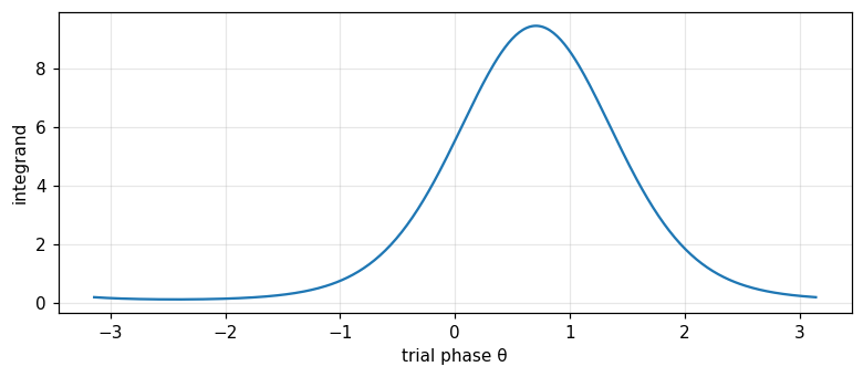
Averaging the likelihood ratio over \theta uniform on [-\pi,\pi] gives \frac{1}{2\pi}\int_{-\pi}^\pi\exp\left[\frac{2A}{N_0}(y_c\cos\theta-y_s\sin\theta)\right]d\theta — exactly the integral definition of the modified Bessel function of order 0: \frac1{2\pi}\int_{-\pi}^\pi e^{a\cos x+b\sin x}\,dx=I_0(\sqrt{a^2+b^2}) (Barkat, pp. 584 to 585). The result: \Lambda=e^{-A^2T/2N_0}I_0\!\left(\frac{2A}{N_0}\sqrt{y_c^2+y_s^2}\right).

The test needs only the envelope r: the incoherent matched filter

Since I_0(\cdot) is monotonically increasing, the test \Lambda\gtrless\eta is equivalent to r=\sqrt{y_c^2+y_s^2}\gtrless\gamma_2 — needing only the envelope of the two quadrature components, without knowing the true phase \Theta (Barkat, pp. 585 to 587). Realized with matched filters (or correlators) against \cos\omega_ct and \sin\omega_ct, squaring each branch, summing, then comparing to a threshold — called the incoherent matched filter or the quadrature receiver.

Measured: the phase-averaged integral matches the closed Bessel function

Measured: with A=1.5, N_0=1, true signal phase \theta=0.7 rad, computing y_c,y_s from a sample signal segment, then r=\sqrt{y_c^2+y_s^2}. The direct numerical integral \frac1{2\pi}\int_{-\pi}^\pi\exp\left[\frac{2A}{N_0}(y_c\cos\theta-y_s\sin\theta)\right]d\theta gives 2.7172, matching the closed Bessel function value I_0(2Ar/N_0) = 2.7172 — confirming the I_0 formula is correct, needing no further assumption beyond its integral definition.

Self-check, part 5

• How does an \"unwanted\" parameter differ from a fully known-in-advance parameter?
• Averaging the likelihood ratio over a uniformly random phase leads to what special function?
• What quantity of the received signal does the incoherent matched filter need, without knowing the true phase?

Hints: its value is not known in advance, only its probability density (random); the modified Bessel function of order 0, I_0; the envelope r=\sqrt{y_c^2+y_s^2} of the two quadrature components.

Takeaways

• The Karhunen–Loève expansion reduces continuous waveform detection in white noise to a finite-dimensional Gaussian problem; for simple binary detection, only one dimension (Y_1) carries information — exactly Example 5.1.
• General binary detection reduces exactly to module 24's equal-covariance problem: d^2=2(E_1+E_0-2\rho\sqrt{E_1E_0})/N_0; antipodal signals (\rho=-1) are always optimal.
• M-ary detection with equal priors reduces MAP to ML (minimum distance); equal-energy orthogonal signals give the "largest of" receiver, the error probability computed by a nested integral of independent Gaussian densities.
• Linear estimation of \theta s(t) reuses exactly the Karhunen–Loève technique, giving \hat\theta_{ml}=Y_1/\sqrt E — a correlator, unbiased, attaining the Cramér–Rao bound N_0/(2E).
• With a random phase (an unwanted parameter), averaging the likelihood ratio gives the Bessel function I_0; the optimal test needs only the envelope r=\sqrt{y_c^2+y_s^2} — the incoherent matched filter.

References

M. Barkat, Signal Detection and Estimation, 2nd ed., Artech House, 2005, chapter 10 (pp. 533 to 590).
Works cited by the chapter: D. O. North (the matched filter, 1943); K. Karhunen, M. Loève (the orthogonal expansion, 1940s); H. L. Van Trees, Detection, Estimation, and Modulation Theory.
The content was written with AI assistance (Claude) and then checked. Every number is produced by a Jupyter notebook and cross-checked by two independent methods; page citations come from the OCR text of the two source books. Mistakes may remain, so please report them.
R. N. Bracewell, The Fourier Transform and Its Applications, 3rd ed., McGraw-Hill, 2000.
M. Barkat, Signal Detection and Estimation, 2nd ed., Artech House, 2005.
This site only summarises, explains and checks numbers; please read the original books through a library or the publisher.
Contribute
Report errors, suggest modules or translations in the GitHub repository, and fork or clone it for your own study. Please credit the source when sharing.