Adaptive thresholding: CFAR detection

Adaptive thresholding: CFAR detection

• Explain why a fixed threshold fails when the background noise variance is unknown or changes over time, and quantify P_F's sensitivity.
• Derive the CA-CFAR detector from the maximum likelihood estimate of the background variance via reference cells, and compute closed-form P_F,P_D.
• Describe the general chi-square-family density of the Swerling target models, and recognise Rayleigh at k=1.
• Explain the masking effect and the capture effect at a clutter edge, and how GO-CFAR, SO-CFAR remedy each case.
• Derive the optimal thresholds for distributed CFAR via a Lagrange multiplier, and compute the global P_D,P_F under the AND, OR fusion rules.

Use the buttons, the dots or the ← → keys to move between slides.

Clutter: unwanted signal from the environment

In real radar detection, the target is buried in thermal noise plus clutter — the term for any unwanted radar signal from scatterers that are not the target of interest: terrain, sea, rain, birds, insects, chaff (Barkat, pp. 627 to 628). Since the radar's operating environment depends on weather and location, the returned signal is statistically nonstationary, with an unknown variance at the receiver input.

A fixed threshold: a dangerously sensitive denominator

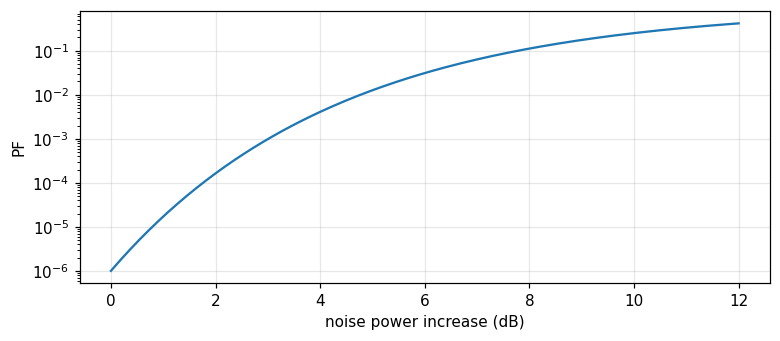
With a single pulse and fixed threshold \gamma, the false-alarm probability is P_F=\exp(-\gamma^2/2\sigma^2), with \sigma^2 the total noise variance (thermal plus clutter) (Barkat, pp. 627 to 628). Let P_{Fd} be the design false-alarm probability for a design variance \sigma_d^2; if the actual variance \sigma^2 differs from \sigma_d^2, P_F=P_{Fd}^{(\sigma_d^2/\sigma^2)}.

Measured: a 3 dB noise-power rise, P_F up more than 1000-fold

With P_{Fd}=10^{-6}, just a 3 dB noise-power increase (i.e. \sigma^2/\sigma_d^2\approx2) makes the actual P_F rise more than 1000-fold — entirely unacceptable for data processing, whether by computer or human operator (Barkat, pp. 628 to 629, Fig. 11.1). Measured: with P_{Fd} = 1.0e-06, a 3 dB rise gives an actual P_F = 1.0000e-03, a ratio increase of 1000-fold.

Radar structure and where the CFAR processor sits

Radar (RAdio Detection And Ranging) transmits electromagnetic energy and extracts target information from the returned echo: range from time delay, direction from a directive antenna, velocity from Doppler shift. The signal processor, sitting between the receiver and the data processor, performs pulse compression, Doppler clutter suppression, and CFAR processing — the CFAR circuit keeps the false-alarm rate constant and relatively low, avoiding saturating the system or the operator (Barkat, pp. 629 to 631).

The core idea: estimate the local noise from neighbouring cells

Finn and Johnson proposed using a reference channel: the range cells surrounding the cell under test are used as reference cells, giving a local estimate of the background noise level, from which the decision threshold is adjusted (Barkat, pp. 634 to 635). This is exactly the CFAR (constant false alarm rate) idea: the threshold \"adapts\" to the changing environment, instead of being fixed.

Self-check, part 1

• What is clutter in the radar context?
• With a fixed threshold, what happens to P_F when the noise variance rises slightly?
• What is the core idea of CFAR?

Hints: an unwanted radar signal from non-target scatterers; P_F rises by orders of magnitude; estimate the local noise from neighbouring reference cells, automatically adjusting the threshold.

The detector structure: a delay line and reference cells

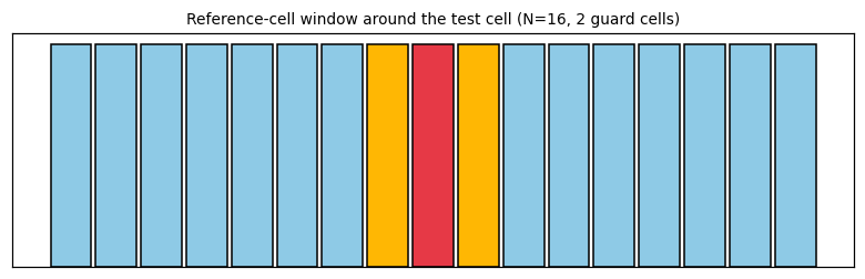
The square-law detector's output feeds a tapped delay line forming the reference cells. To avoid signal energy spilling from the test cell into adjacent cells and biasing the clutter estimate, the cells immediately adjacent — called guard cells — are entirely ignored. The reference window U (the sum of N/2 leading cells) and V (the sum of N/2 lagging cells) are added to give Z=U+V, the clutter-level estimate (Barkat, pp. 635 to 637, Figs. 11.11, 11.12).

The statistical model: exponential under both hypotheses

With a slowly fluctuating Swerling case 1 target buried in white Gaussian noise, the square-law detector output of the test cell has an exponential density: f_{Y|H_1}(y|H_1)=\frac{1}{2\sigma^2(1+S)}\exp\!\left[-\frac{y}{2\sigma^2(1+S)}\right], f_{Y|H_0}(y|H_0)=\frac{1}{2\sigma^2}\exp(-\frac{y}{2\sigma^2}), with S the target signal-to-noise ratio (Barkat, pp. 637 to 638). The reference cells X_i are independent, identically exponentially distributed as H_0.

Z is Gamma (N,2\sigma^2): a neat closed-form P_F

The sum of N independent identically exponential variables is a Gamma(N,2\sigma^2) variable, with moment generating function M_Z(t)=(1-2\sigma^2t)^{-N} (Barkat, pp. 638 to 639). From P_D=E_Z[P(Y>TZ|Z,H_1)]=M_Z[T/2\sigma^2(1+S)] and setting S=0 for P_F: P_F=M_Z(T/2\sigma^2)=(1+T)^{-N} — no longer depending on the unknown \sigma^2! Inverting gives the threshold multiplier T=P_F^{-1/N}-1.

The detection probability: the Neyman–Pearson bound as N\to\infty

Substituting T/2\sigma^2 by T/[2\sigma^2(1+S)] in the P_F formula gives P_D=\left[\dfrac{1+S}{1+S+T}\right]^N (Barkat, p. 639). For a homogeneous noise background, CA-CFAR is optimal in the sense that its P_D approaches that of the ideal Neyman–Pearson detector (which knows \sigma^2) as the reference-cell count N\to\infty — there is always a finite CFAR loss for finite N, traded for not needing to know \sigma^2.

Measured: T, P_F, P_D match a Monte Carlo simulation

Measured: with N=16, design P_{Fd}=10^{-4}: the threshold multiplier T = 0.7783. A Monte Carlo simulation of 2 million trials (generating N exponential reference samples and one test sample): the measured P_F is 9.90e-05, matching the design 1.0e-04. With S=5: the theoretical P_D=[(1+S)/(1+S+T)]^N = 0.1421, matching the simulated 0.1413.

Self-check, part 2

• What is the role of the guard cells?
• Why does P_F=1/(1+T)^N no longer depend on \\sigma^2?
• What performance does CA-CFAR's P_D approach as N\\to\\infty?

Hints: to avoid signal energy from the test cell spilling over and biasing the clutter estimate; because \sigma^2 cancels in the ratio T/2\sigma^2 when substituted into the Gamma moment generating function; the performance of the ideal Neyman–Pearson detector (knowing \sigma^2).

Why the radar cross section is not a constant

The radar cross section (RCS) is the effective scattering area of a target as seen by the radar. Since a target is made of many scattering elements, and the return from each depends on the illumination angle, frequency, wave polarisation, and target motion and vibration, the RCS fluctuates over time (Barkat, p. 640). The fluctuation effect requires a higher signal-to-noise ratio to reach a high detection probability, compared with a nonfluctuating signal.

A scan and the four Swerling cases

A scan is when the antenna's main beam completes one search of the surveillance region. Slow fluctuation, scan to scan (but constant within one pulse group) is called scan-to-scan; fast fluctuation, changing pulse to pulse within the group, is called pulse-to-pulse. Case 1 (scan-to-scan, Rayleigh) and 2 (pulse-to-pulse, Rayleigh) correspond to a target of many independent scattering elements, none dominant (like a large aircraft); Cases 3, 4 correspond to one dominant element plus other small ones (like a missile) (Barkat, pp. 640 to 641).

The general chi-square-family density P_k(S)

All Swerling Cases 1 to 4 unify into one family: P_k(S)=\dfrac1{\Gamma(k)}\left(\dfrac{k}{m_s}\right)^kS^{k-1}\exp\!\left(-\dfrac{kS}{m_s}\right), S\ge0, with m_s the average signal-to-noise ratio, k=m_s^2/\text{var}[S] (Barkat, pp. 641 to 642). Cases 1, 2 (Rayleigh) correspond to k=1; Cases 3, 4 (one-dominant-plus-Rayleigh) correspond to k=2; Case 5 (nonfluctuating) corresponds to k\to\infty.

Measured: the density normalises and the mean matches m_s

Measured: with m_s=3, the numerical integral of P_k(S) over [0,\infty) gives 1 at k=1 and 1 at k=2 (both near 1, confirming correct normalisation). The numerically integrated mean \int SP_k(S)\,dS gives 3 at k=1 and 3 at k=2 — both matching the set m_s=3, exactly as m_s's definition requires.

Why the target model matters for CFAR design

The formula P_D=[(1+S)/(1+S+T)]^N of part 2 assumes S is a known constant — in fact S is random under a Swerling model. For Case 1 (used in part 2), the actual P_D needs averaging over P(S) of (11.20) across the whole range of S; for other cases, the corresponding P_k(S) is needed. Choosing the wrong target model (e.g. using k=1 for a target that is actually k=2) biases the predicted P_D away from the system's actual performance.

Self-check, part 3

• How does scan-to-scan fluctuation differ from pulse-to-pulse?
• What value of k corresponds to a Rayleigh target (many independent scattering elements)?
• What value of k corresponds to Swerling Case 5 (nonfluctuating)?

Hints: scan-to-scan changes between scans but not within a pulse group, pulse-to-pulse changes with every pulse; k=1; k\to\infty.

The clutter-edge model: a step in clutter power

A real environment cannot be described by a single clutter model. A homogeneous background means the reference cells are independent and identically distributed; a clutter edge describes a situation with a step transition in clutter power against range — like a rain-area boundary (Barkat, pp. 642 to 644, Fig. 11.14). Two serious scenarios can occur depending on the edge's position relative to the test cell and the reference window.

Masking: a clear test cell, clutter-contaminated reference

If the test cell lies in the clear region but some reference cells lie in clutter, CA-CFAR's estimate Z=U+V is inflated, pulling the threshold higher than necessary — reducing P_D and P_F in the clear region. This is called the masking effect: a real target may go undetected even though it lies in a clear region, simply because neighbouring cells (not the test cell) are clutter-contaminated (Barkat, p. 643).

Capture: a test cell in clutter, partly clear reference

Conversely, if the test cell lies in clutter but some reference cells lie in the clear region, CA-CFAR's estimate is pulled too low — the threshold becomes too low, making the false-alarm probability rise unacceptably. Hansen and Sawyers proposed GO-CFAR (greatest-of, choosing the larger of U,V) to restrain this situation (Barkat, pp. 643 to 644).

SO-CFAR: remedying masking when multiple targets are present

Weiss showed that when one or more interfering targets are present in the reference cells, GO-CFAR performs poorly; Trunk proposed SO-CFAR (smallest-of, choosing the smaller of U,V) to handle this, helping preserve target resolution better (Barkat, p. 644). Intuition: when the test cell is clear but half the reference is clutter-contaminated (masking), choosing the cleaner half (\min) as the noise estimate avoids the threshold being pulled up by the contaminated half.

Measured: each variant remedies exactly its own scenario

Measured (masking scenario, N=16, S=8, P_{Fd}=10^{-3}, half the reference in clutter of 3x power, clear test cell): nominal P_D (no clutter) = 0.3937; CA-CFAR gives P_D = 0.1668 (masked, markedly lower); SO-CFAR gives P_D = 0.4051 (close to nominal). Capture scenario (test cell in clutter, half the reference clear): CA-CFAR gives P_F = 0.0085 (blown up against the design 1.0e-03); GO-CFAR gives P_F = 0.0025 (markedly better restrained).

Self-check, part 4

• In what situation does the masking effect occur?
• Which value between U and V does GO-CFAR choose as the noise estimate?
• In what situation is SO-CFAR more suitable than GO-CFAR?

Hints: the test cell is clear but part of the reference is clutter-contaminated; the larger value \max(U,V); when the test cell is clear but the reference is partly clutter-contaminated (masking) or has interfering targets.

Why distributed detection is needed

With a wide surveillance area or many targets, several geographically distributed receivers observe the same phenomenon. Instead of transmitting all the raw data to a central processor (bandwidth-costly), each sensor processes locally and sends only a binary decision D_i\in\{0,1\} to a data fusion center, where the local decisions are combined by a fusion rule to give the global decision D_0 (Barkat, pp. 665 to 666).

Each sensor is a CA-CFAR with its own threshold

Barkat and Varshney developed the theory of distributed CA-CFAR for a Swerling 1 target in white Gaussian noise of unknown level. The local detection probability at sensor i is P_{Di}=\left[\dfrac{1+S}{1+S+T_i}\right]^{N_i} — exactly the CA-CFAR formula of part 2, with an index i added per sensor (Barkat, pp. 666 to 667).

Optimising the thresholds via a Lagrange multiplier

The goal: maximise the global P_D while keeping the global P_F at a fixed value \alpha. Form the objective function J(T_1,\ldots,T_N)=P_D+\lambda[P_F-\alpha], solve the system \partial J/\partial T_j=0, j=1,\ldots,N, for the optimal threshold multipliers \{T_i\} (Barkat, pp. 667 to 668) — exactly the Lagrange-multiplier technique met in the Neyman–Pearson test (module 21).

The AND and OR rules: combining local decisions

With the AND rule (the global decision is H_1 only if every sensor decides H_1), since the sensors are independent: P_D=\prod_{i=1}^NP_{Di}, P_F=\prod_{i=1}^NP_{Fi} (Barkat, pp. 668 to 669). With the OR rule (just one sensor deciding H_1 suffices): P_D=1-\prod_{i=1}^N(1-P_{Di}), P_F=1-\prod_{i=1}^N(1-P_{Fi}). The AND rule gives a global P_D,P_F smaller than each local P_{Di},P_{Fi}; the OR rule gives larger.

Measured: the AND, OR formulas match an independent simulation

Measured: with two independent sensors, P_{D1}=0.8, P_{D2}=0.7, P_{F1}=0.01, P_{F2}=0.02: the AND rule gives P_D = 0.56 (theory) matching a Monte Carlo simulation of 2 million trials 0.5602, and P_F = 0.0002 matching 0.0002. The OR rule gives P_D = 0.94 matching 0.9397, and P_F = 0.0298 matching 0.0298 — confirming both product formulas hold for an independent system.

Looking back: from a single cell to a sensor network

The whole chapter builds layer by layer: a fixed threshold fails (part 1) → CA-CFAR's local noise estimate solves that (part 2) → the Swerling target model makes P_D more accurate (part 3) → GO/SO-CFAR handle when the homogeneity assumption is violated (part 4) → distributed CFAR extends the whole idea to a network of sensors (part 5). Each layer solves exactly one limitation of the layer before it.

Self-check, part 5

• Why do distributed sensors send a binary decision instead of raw data?
• Does the AND rule give a global P_D,P_F larger or smaller than each local value?
• What is the Lagrange-multiplier technique used for in distributed CFAR?

Hints: to save communication bandwidth between the sensors and the center; smaller (the product of probabilities below 1); to maximise the global P_D while keeping the global P_F fixed.

Takeaways

• With a fixed threshold, P_F=\exp(-\gamma^2/2\sigma^2) is extremely sensitive to the unknown noise variance; a rise of just a few dB makes P_F jump by thousands — an adaptive threshold is needed.
• CA-CFAR estimates the background noise from the sum of N reference cells (Gamma distributed), giving P_F=1/(1+T)^N independent of \sigma^2, and P_D=[(1+S)/(1+S+T)]^N approaching the ideal performance as N\to\infty.
• The Swerling target models unify into the chi-square family P_k(S): k=1 (Rayleigh, many independent scatterers), k=2 (one-dominant-plus-Rayleigh); further distinguished as scan-to-scan or pulse-to-pulse.
• At a clutter edge, masking (clear test cell, contaminated reference) and capture (the reverse) make CA-CFAR fail; SO-CFAR (min) remedies masking, GO-CFAR (max) remedies capture.
• Distributed CFAR optimises each sensor's threshold via a Lagrange multiplier; the AND rule gives a global P_D,P_F as the product of local values (smaller), the OR rule gives 1-\prod(1-\cdot) (larger).

References

M. Barkat, Signal Detection and Estimation, 2nd ed., Artech House, 2005, chapters 11 and 12 (pp. 627 to 670).
Works cited by the chapter: H. M. Finn and R. S. Johnson (CA-CFAR); P. Swerling (the target model, 1950s); V. G. Hansen and J. H. Sawyers (GO-CFAR); G. V. Trunk, M. Weiss (SO-CFAR); M. Barkat and P. K. Varshney (distributed CFAR).
The content was written with AI assistance (Claude) and then checked. Every number is produced by a Jupyter notebook and cross-checked by two independent methods; page citations come from the OCR text of the two source books. Mistakes may remain, so please report them.
R. N. Bracewell, The Fourier Transform and Its Applications, 3rd ed., McGraw-Hill, 2000.
M. Barkat, Signal Detection and Estimation, 2nd ed., Artech House, 2005.
This site only summarises, explains and checks numbers; please read the original books through a library or the publisher.
Contribute
Report errors, suggest modules or translations in the GitHub repository, and fork or clone it for your own study. Please credit the source when sharing.